\(\renewcommand\AA{\unicode{x212B}}\)

LoadWANDSCD v1

Enable screenshots using DOCS_SCREENSHOTS in CMake

Summary

Load WAND single crystal data into a detector space vs rotation MDHisto

See Also

ConvertWANDSCDtoQ

Properties

Name	Direction	Type	Default	Description
Filename	Input	list of str lists		Files to load. Allowed extensions: [‘.nxs.h5’]
IPTS	Input	long	Optional	IPTS number to load from
RunNumbers	Input	long list		Run numbers to load
VanadiumIPTS	Input	long	Optional	IPTS number to load Vanadium normalization
VanadiumRunNumber	Input	long	Optional	Run number to load Vanadium normalization
VanadiumFile	Input	string		File with Vanadium normalization scan data. Allowed extensions: [‘.nxs’]
VanadiumWorkspace	Input	IMDHistoWorkspace		MDHisto workspace containing vanadium normalization data
NormalizedBy	Input	string	None	Normalize to Counts, Monitor, Time. Allowed values: [‘None’, ‘Counts’, ‘Monitor’, ‘Time’]
Grouping	Input	string	None	Group pixels (shared by input and normalization). Allowed values: [‘None’, ‘2x2’, ‘4x4’]
OutputWorkspace	Output	Workspace	Mandatory	Output Workspace

Description

This algorithm will load a series of runs into a MDHistoWorkspace that has dimensions x and y detector pixels vs scanIndex. The scanIndex is the omega rotation of the sample. The instrument attached to the OutputWorkspace is directly copied from the FIRST run, therefore it is crucial to have the correct instrument attached to the first run. In addition the s1 (omega rotation), duration, run_number and monitor count is read from every file and included in the logs of the OutputWorkspace.

During a recent feature expansion, normalization can be optionally performed in the same process provided that the necessary Vanadium data is specified. By default, the algorithm will try to locate the Vanadium data using IPTS and run number. If failed, it will check the Vanadium filename entry to see if the data can be loaded directly from file. If neither is provided, the algorithm will try to check if the Vanadium data is provided as a workspace in memory. Currently there are three normalization scheme supported: by Count, by Monitor and by Time. If None is selected, no normalization will be performed and all normalization related properties will be ignored (on the GUI end, they will be disabled instead).

If the “HB2C:CS:CrystalAlign:UBMatrix” property exist, it will be converted into the OrientedLattice on the OutputWorkspace. The goniometer tilts (sgu and sgl) are combined into the UB Matrix so that only omega (s1) needs to be taken into account during rotation.

This algorithm doesn’t use Mantid loaders but instead h5py and numpy to load and integrate the events.

There is a grouping option to group pixels by either 2x2 or 4x4 which will help in reducing memory usage and speed up the later reduction steps. In most cases you will not see a difference in reduced data with 4x4 pixel grouping. Also, both input data and the Vanadium data will share the same grouping scheme.

The loaded workspace is designed to be the input to ConvertWANDSCDtoQ v1.

Usage

Load one file, Vanadium for normalisation

norm = LoadWANDSCD(IPTS=7776, RunNumbers=26509)
print(repr(norm))

Output:

MDHistoWorkspace
Title:
Dim 0: (y) 0.5 to 512.5 in 512 bins
Dim 1: (x) 0.5 to 3840.5 in 3840 bins
Dim 2: (scanIndex) 0.5 to 1.5 in 1 bins

Inelastic: ki-kf
Instrument: ...

Run start: 2018-Mar-12 17:10:59
Run end:  not available
Sample: a 1.0, b 1.0, c 1.0; alpha 90, beta 90, gamma 90

Load data and Vanadium at the same time

data = LoadWANDSCD(
    IPTS=7776, RunNumbers='26640-27944',
    VanadiumIPTS=7776, VanadiumRunNumber=26509,
    NormalizedBy='Monitor',
    )

Load multiple data file

data = LoadWANDSCD(IPTS=7776, RunNumbers='26640-27944')
print("Memory used: {}GiB".format(data.getMemorySize()/2**30))
print(repr(data))
print('s1 = {}'.format(data.getExperimentInfo(0).run().getProperty('s1').value[0:10]))
print('monitor_counts = {}'.format(data.getExperimentInfo(0).run().getProperty('monitor_counts').value[0:10]))
print('duration = {}'.format(data.getExperimentInfo(0).run().getProperty('duration').value[0:10]))
print('run_number = {}'.format(data.getExperimentInfo(0).run().getProperty('run_number').value[0:10]))

Output:

Memory used: 59GB

MDHistoWorkspace
Title:
Dim 0: (y) 0.5 to 512.5 in 512 bins
Dim 1: (x) 0.5 to 3840.5 in 3840 bins
Dim 2: (scanIndex) 0.5 to 1305.5 in 1305 bins
Inelastic: ki-kf
Instrument: ...
Run start: 2018-May-02 13:34:10
Run end:  not available
Sample: a 5.7, b 5.7, c 5.6; alpha 93, beta 90, gamma 98

s2 = [-180,-179.9,-179.8,-179.7,-179.6,-179.5,-179.4,-179.3,-179.2,-179.1]
monitor_count = [44571,44598,44567,44869,44453,44238,44611,44120,44762,44658]
duration = [2.05,2.05,2.03333,2.05,2.03333,2.03333,2.05,2.01667,2.05,2.05]
run_number = [26640,26641,26642,26643,26644,26645,26646,26647,26648,26649]

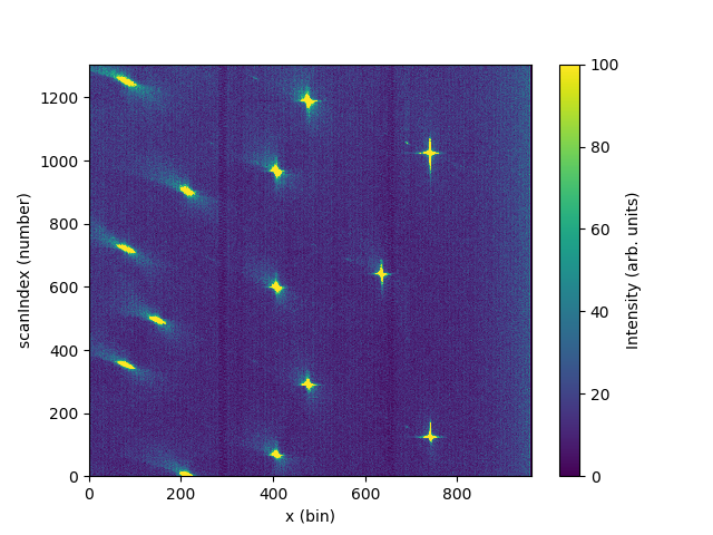
Load with different grouping comparing memory usage

data = LoadWANDSCD(IPTS=7776, RunNumbers='26640-27944')
data_2x2 = LoadWANDSCD(IPTS=7776, RunNumbers='26640-27944', Grouping='2x2')
data_4x4 = LoadWANDSCD(IPTS=7776, RunNumbers='26640-27944', Grouping='4x4')
print("Memory used by {}: {}GiB".format(data,data.getMemorySize()/2**30))
print("Memory used by {}: {}GiB".format(data_2x2,data_2x2.getMemorySize()/2**30))
print("Memory used by {}: {}GiB".format(data_4x4,data_4x4.getMemorySize()/2**30))
print(repr(data_4x4))

# Integrate y and plot
data_integrated = IntegrateMDHistoWorkspace('data_4x4', P1Bin='0,129')
import matplotlib.pyplot as plt
from mantid import plots
fig, ax = plt.subplots(subplot_kw={'projection':'mantid'})
c = ax.pcolormesh(data_integrated, vmax=100)
cbar=fig.colorbar(c)
cbar.set_label('Intensity (arb. units)')
#fig.savefig('LoadWANDSCD.png')

Output:

Memory used by data: 59GiB
Memory used by data_2x2: 14GiB
Memory used by data_4x4: 3GiB

MDHistoWorkspace
Title:
Dim 0: (y) 0.5 to 128.5 in 128 bins
Dim 1: (x) 0.5 to 960.5 in 960 bins
Dim 2: (scanIndex) 0.5 to 1305.5 in 1305 bins
Inelastic: ki-kf
Instrument: ...
Run start: 2018-May-02 13:34:10
Run end:  not available
Sample: a 5.7, b 5.7, c 5.6; alpha 93, beta 90, gamma 98

Categories: AlgorithmIndex | DataHandling\Nexus

Source

Python: LoadWANDSCD.py