\(\renewcommand\AA{\unicode{x212B}}\)

DiscusMultipleScatteringCorrection v1

Summary

Calculates a multiple scattering correction using a Monte Carlo method

See Also

MayersSampleCorrection, CarpenterSampleCorrection, VesuvioCalculateMS

This algorithm is also known as: Muscat

Properties

Name	Direction	Type	Default	Description
InputWorkspace	Input	MatrixWorkspace	Mandatory	The name of the input workspace. The input workspace must have X units of Momentum (k) for elastic calculations and units of energy transfer (DeltaE) for inelastic calculations. This is used to supply the sample details, the detector positions and the x axis range to calculate corrections for
StructureFactorWorkspace	Input	Workspace	Mandatory	The name of the workspace containing S’(q) or S’(q, w). For elastic calculations, the input workspace must contain a single spectrum and have X units of momentum transfer. A workspace group containing one workspace per component can also be supplied if a calculation is being run on a workspace with a sample environment specified
OutputWorkspace	Output	WorkspaceGroup	Mandatory	Name for the WorkspaceGroup that will be created. Each workspace in the group contains a calculated weight for a particular number of scattering events. The number of scattering events varies from 1 up to the number supplied in the NumberOfScatterings parameter. The group will also include an additional workspace for a calculation with a single scattering event where the absorption post scattering has been set to zero
ScatteringCrossSection	Input	MatrixWorkspace		A workspace containing the scattering cross section as a function of k, \(\sigma_s(k)\). Note - this parameter would normally be left empty which results in the tabulated cross section data being used instead which implies no wavelength dependence
NumberOfSimulationPoints	Input	number	Optional	The number of points on the input workspace x axis for which a simulation is attempted
NeutronPathsSingle	Input	number	1000	The number of “neutron” paths to generate for single scattering
NeutronPathsMultiple	Input	number	1000	The number of “neutron” paths to generate for multiple scattering
SeedValue	Input	number	123456789	Seed the random number generator with this value
NumberScatterings	Input	number	2	Number of scatterings
Interpolation	Input	string	Linear	Method of interpolation used to compute unsimulated values. Allowed values: [‘Linear’, ‘CSpline’]
SparseInstrument	Input	boolean	False	Enable simulation on special instrument with a sparse grid of detectors interpolating the results to the real instrument.
NumberOfDetectorRows	Input	number	5	Number of detector rows in the detector grid of the sparse instrument.
NumberOfDetectorColumns	Input	number	10	Number of detector columns in the detector grid of the sparse instrument.
ImportanceSampling	Input	boolean	False	Enable importance sampling on the Q value chosen on multiple scatters based on Q.S(Q)
MaxScatterPtAttempts	Input	number	5000	Maximum number of tries made to generate a scattering point within the sample. Objects with holes in them, e.g. a thin annulus can cause problems if this number is too low. If a scattering point cannot be generated by increasing this value then there is most likely a problem with the sample geometry.
SimulateEnergiesIndependently	Input	boolean	False	For inelastic calculation, whether the results for adjacent energy transfer bins are simulated separately. Currently applies to Direct geometry only
NormalizeStructureFactors	Input	boolean	False	Enable normalization of supplied structure factor(s). May be required when running a calculation involving more than one material where the normalization of the default S(Q)=1 structure factor doesn’t match the normalization of a supplied non-isotropic structure factor

Description

This algorithm calculates a Multiple Scattering correction using a Monte Carlo integration method. The method uses a structure function for the sample to determine the probability of a particular momentum transfer (q) and energy transfer (\(\omega\)) value for each scattering event and it doesn’t therefore rely on an assumption that the scattering is isotropic.

The structure function that the algorithm takes as input is a linear combination of the coherent and incoherent structure factors:

\(S'(Q, \omega) = \frac{1}{\sigma_b}(\sigma_{coh} S(Q, \omega) + \sigma_{inc} S_s(Q, \omega))\)

If the sample is a perfectly coherent scatterer then \(S'(Q, \omega) = S(Q, \omega)\)

The algorithm is based on code which was originally written in Fortran as part of the Discus program [1]. The code was subsequently resurrected and improved by Spencer Howells under the Muscat name and was included in the QENS MODES package [2], [3] These original programs calculated multiple scattering corrections for inelastic instruments but an elastic diffraction version of the code was also created and results from that program are included in this paper by Mancinelli [4].

Theory

The theory is outlined here for an inelastic calculation. The calculation performed for an elastic instrument is a special case of this with \(\omega=0\).

The algorithm calculates a set of dimensionless weights \(J_n\) describing the probability of detection at an angle \(\theta\) after n scattering events given a total incident flux \(I_0\) and a transmitted flux of T:

\(T_n(\theta,k_{in}, \omega) = J_n(\theta,k_{in}, \omega) I_0(k_{in})\)

The quantity \(J_n\) is calculated by performing the following integration:

\[\begin{split}J_n &= (\frac{\mu_s}{4 \pi})^n \frac{1}{A} \int dS \int_{0}^{l_1^{max}} dl_1 e^{-\mu_T l_1} \prod\limits_{i=1}^{n-1} [\int_{0}^{l_{i+1}^{max}} dl_{i+1} \int_{0}^{\pi} \sin\theta_i d\theta_i \int_{0}^{2 \pi} d\phi_i \int_{\omega^{min}}^{\omega_i^{max}} d\omega_i (e^{-\mu_T l_{i+1}}) \frac{k_{i+1}}{k_i} S(Q_i, \omega_i)] e^{-\mu_T l_{out}} S(Q_n, \omega_n) \\ &=(\frac{\mu_s}{4 \pi})^n \frac{1}{A} \int dS \int_{0}^{l_1^{max}} dl_1 e^{-\mu_T l_1} \prod\limits_{i=1}^{n-1} [\int_{0}^{l_{i+1}^{max}} dl_{i+1} \int_{0}^{2 \pi} d\phi_i \iint \limits_{D(k_i)} dQ_i d\omega_i (e^{-\mu_T l_{i+1}}) \frac{Q_i}{k_i^2} S(Q_i, \omega_i)] e^{-\mu_T l_{out}} S(Q_n, \omega_n)\end{split}\]

The variables \(l_i^{max}\) represent the maximum path length before the next scatter given a particular phi and theta value (Q). Each \(l_i\) is actually a function of all of the earlier values for the \(l_i\), \(\phi\), \(Q\) and \(\omega\) variables ie \(l_i = l_i(l_1, l_2, ..., l_{i-1}, \phi_1, \phi_2, ..., \phi_i, Q_1, Q_2, ..., Q_i, \omega_1, \omega_2, ..., \omega_i)\). The integration over the variables \(Q\) and \(\omega\) is done over the kinematically accessible region \(D(k_i)\). The integral is done over \(\omega\) first and the range is defined by the minimum value on the \(\omega\) axis in the \(S(Q, \omega)\) profile and a maximum which is equal to the total energy loss of the pre-scatter neutron prior to the ith scatter. The limits on the q integration are then calculated as follows (and are also a function of i). These formulae for the q limits reduce to 0 and 2k for elastic.

\(q_i^{min} = |k_{i+1} - k_i|\)

\(q_i^{max} = q_i^{min} + 2 min(k_i, k_{i+1})\)

The following substitutions are then performed in order to make it more convenient to evaluate as a Monte Carlo integral:

\(t_i = \frac{1-e^{-\mu_T l_i}}{1-e^{-\mu_T l_i^{max}}}\)

\(u_i = \frac{\phi_i}{2 \pi}\)

\(2 k_i^2 = \frac{\sigma_s}{\sigma_s(k_i)} I(k_i)\) where \(I(k) = \iint \limits_{D(k)} Q S(Q, \omega) dQ d\omega\)

Using the new variables the integral is:

\[J_n = \frac{1}{A} \int\hspace{-3pt}dS\int_{0}^{1}\hspace{-3pt}dt_1 \frac{1-e^{-\mu_T l_1^{\ max}}}{\sigma_T} \prod\limits_{i=1}^{n-1}[\int_{0}^{1}\hspace{-3pt}dt_{i+1}\int_{0}^{1} du_i \iint \limits_{D(k_i)}\hspace{-3pt}dQ_i d\omega_i\frac{(1-e^{-\mu_T l_{i+1}^{max}})}{\sigma_T} \frac{Q_i S(Q_i, \omega_i)}{I(k_i)} \sigma_s(k_i)] e^{-\mu_T l_{out}} S(Q_n, \omega_n) \frac{\sigma_s}{4 \pi}\]

This is evaluated as a Monte Carlo integration by selecting random values for the variables \(t_i\) and \(u_i\) between 0 and 1. The integral over \(Q\omega\) space is performed by integrating a slightly modified \(S(Q,\omega)\) function over a rectangular region. \(S_{kin}(Q,\omega)\) equals zero if \(Q\) and \(\omega\) are outside the kinematically accessible region. The rectangular region spans the full length of the \(\omega\) axis in the \(S(Q,\omega)\) profile and goes from zero to the maximum possible \(Q_i\) for a particular \(k_i\) in the q direction.

A simulated path is traced through the sample to enable the \(l_i^{\ max}\) values to be calculated. The path is traced by calculating the \(l_i\), \(\theta\) and \(\phi\) values as follows from the random variables. The code keeps a note of the start coordinates of the current path segment and updates it when moving to the next segment using these randomly selected lengths and directions:

\(l_i = -\frac{1}{\mu_T}ln(1-(1-e^{-\mu_T l_i^{\ max}})t_i)\)

\(\cos\theta_i = (k_i^2 + k_{i+1}^2 - Q_i^2)/2 k_i k_{i+1}\)

\(\phi_i = 2 \pi u_i\)

The final Monte Carlo integration that is actually performed by the code is as follows where N is the number of scenarios:

\[J_n = \frac{1}{N}\sum \frac{1-e^{-\mu_T l_1^{\ max}}}{\sigma_T} \prod\limits_{i=1}^{n-1}[\frac{(1-e^{-\mu_T l_{i+1}^{max}})}{\sigma_T} \frac{\Delta Q_i \Delta \omega Q_i S_{kin}(Q_i, \omega_i)}{I(k_i)} \sigma_s(k_i)] e^{-\mu_T l_{out}} S(Q_n, \omega_n) \frac{\sigma_s}{4 \pi}\]

where the integration ranges over the rectangular \(Q \omega\) region are defined as follows:

\(\Delta\omega = \omega^{max}-\omega^{min}\)

\(\Delta Q_i = k_i + \frac{2m}{\hbar}\sqrt{\frac{\hbar^2 k_i^2}{2m} - \omega_{min}}\)

This is similar to the formulation described in the Mancinelli paper except there is no random variable to decide whether a particular scattering event is coherent or incoherent.

The integral \(I(k)\) is evaluated deterministically up front at a set of k values and interpolated as required.

The factor for the final track segment can also be normalised by setting NormalizeStructureFactors=true which replaces \(\sigma_s\) with \(2k_n^2 \sigma_s(k_n)/I(k_n)\). This feature wasn’t in the original Discus implementation.

The results for different \(\omega\) values can be calculated by simulating tracks separately for each \(\omega\) value or the same tracks can be reused with the multiple weights for the final track segment being calculated to achieve the required range of overall energy transfers. Discus used the latter approach which results in the results for different \(\omega\) being correlated. This choice is controlled using the SimulateEnergiesIndependently parameter

Importance Sampling

The algorithm includes an option to use importance sampling to improve the results for elastic instrument when running with S(Q) profiles containing spikes. Without this option enabled, the contribution from rare, high values in the structure factor is only visible at a very high number of scenarios.

The importance sampling is achieved using a further change of variables as follows:

\(v_i = P(Q_i) = \frac{I(Q_i)}{I(2k)}\) where \(I(x) = \int_{0}^{x} Q S(Q) dQ\)

With this approach the Q value for each segment is chosen as follows based on a \(v_i\) value randomly selected between 0 and 1:

\(Q_i = P^{-1}(v_i)\)

\(\cos\theta_i\) is determined from \(Q_i\) as before. The change of variables gives the following integral for \(J_n\):

\[ \begin{align}\begin{aligned}J_n = \frac{1}{A} \int dS \int_{0}^{1} dt_1 \frac{1-e^{-\mu_T l_1^{\ max}}}{\sigma_T} \prod\limits_{i=1}^{n-1}[\int_{0}^{1} dt_{i+1} \int_{0}^{1} dv_i \frac{I(2k)}{2k^2} \sigma_s \int_{0}^{1} du_i \frac{(1-e^{-\mu_T l_{i+1}^{max}})}{\sigma_T}] e^{-\mu_T l_{out}} S(Q_n) \frac{\sigma_s}{4 \pi}\\J_n = \frac{1}{A} \int dS \int_{0}^{1} dt_1 \frac{1-e^{-\mu_T l_1^{\ max}}}{\sigma_T} \prod\limits_{i=1}^{n-1}[\int_{0}^{1} dt_{i+1} \int_{0}^{1} dv_i \sigma_s(k) \int_{0}^{1} du_i \frac{(1-e^{-\mu_T l_{i+1}^{max}})}{\sigma_T}] e^{-\mu_T l_{out}} S(Q_n) \frac{\sigma_s}{4 \pi}\end{aligned}\end{align} \]

Finally, the equivalent Monte Carlo integration that the algorithm performs with importance sampling enabled is:

\[J_n = \frac{1}{N}\sum \frac{1-e^{-\mu_T l_1^{\ max}}}{\sigma_T} \prod\limits_{i=1}^{n-1}[\sigma_s(k) \frac{(1-e^{-\mu_T l_{i+1}^{max}})}{\sigma_T}] e^{-\mu_T l_{out}} S(Q_n) \frac{\sigma_s}{4 \pi}\]

The importance sampling has also been implemented for inelastic instruments by flatting out the 2D \(S(Q, \omega)\) profile into a 1D array. A 1D coordinate is created which is the actual Q value added onto the maximum Q from the preceding \(\omega\) row: \(Q'(Q,\omega_i) = Q + Q_{max}(\omega_{i-1})\) With this approach there is no interpolation performed between different \(\omega\) values. It’s not clear whether the importance sampling is useful for inelastic calculations since the area where the multiple scattering correction tends to be largest relative to the signal is away from the peak in \(S(Q, \omega)\).

Support for sample environment

The calculation can include scattering from the sample environment (e.g. can) in the Monte Carlo simulation. The term “segment” has previously been used to refer to a straight neutron path between two scattering events. For the purpose of this description the term “link” will be used to refer to a subsection of a segment that lies within a single material.

The modified calculation is illustrated here with an example of a sample contained in a can where a track may contain three different links (can, then sample, then can). If the selected scatter point occurs somewhere in the third link, the quantity \(t_i\) is redefined as:

\[t_i = \frac{1-e^{-\mu_1 l_1^{max} - \mu_2 l_2^{max} - \mu_3 (l_i - l_1^{max} - l_2^{max})}}{1-e^{-\mu_1 l_1^{max} - \mu_2 l_2^{max} - \mu_3 l_3^{max}}}\]

This can be generally expressed as follows where n is the number of sample environment components:

\[t_i = \frac{1-e^{-\sum\limits_{j=1}^{n} \mu_j\ min(max( l_i - \sum\limits_{k=1}^{j-1} l_k^{max},\ 0),\ l_j^{max})}}{1-e^{-\sum\limits_{j=1}^{n} \mu_j l_j^{max}}}\]

Based on this the length of the ith segment can be derived from a \(t_i\) that has been randomly selected between 0 and 1 as follows where again the expression is for the specific case of a track containing three different links:

(1)\[\mu_1 l_1^{max} + \mu_2 l_2^{max} + \mu_3 (l_i - l_1^{max} - l_2^{max}) = - ln(1-(1-e^{-\sum\limits_{j=1}^{n}\mu_j l_j^{max}})t_i)\]

…and more generally (although perhaps less helpfully in terms of explaining how the code works):

\[\sum\limits_{j=1}^{n} \mu_j\ min(max( l_i - \sum\limits_{k=1}^{j-1} l_k^{max},\ 0),\ l_j^{max}) = - ln(1-(1-e^{-\sum\limits_{j=1}^{n}\mu_j l_j^{max}})t_i)\]

It can be seen that the formula (1) can be solved for \(l_i\) by calculating the quantity on the right hand side and then sequentially subtracting \(\mu_i l_i^{max}\) from it for increasing i while keeping the running total >=0. The value of \(i\) when you can’t subtract any more \(\mu_i l_i^{max}\) identifies the component containing the scatter. Dividing by \(\mu_i\) at this point gives you the length into that component that the track reaches.

The other modification to the calculation to support scattering in the sample environment is that a different structure factor \(S(Q,\omega)\) , \(I(k)\) and scattering cross section \(\sigma_s\) is required for each material. The component containing each scatter is derived from the \(l_i\) calculation and is used to look up the material.

Outputs

The algorithm outputs a workspace group containing the following workspaces:

• Several workspaces called Scatter_n where n is the number of scattering events considered. Each workspace contains “per detector” weights as a function of momentum or energy transfer for a specific number of scattering events. The number of scattering events ranges between 1 and the number specified in the NumberOfScatterings parameter

• Several workspaces called Scatter_n_Integrated which are integrals of the Scatter_n workspaces across the x axis (Momentum for elastic and DeltaE for inelastic)

• A workspace called Scatter_1_NoAbsorb is also created for a scenario where neutrons are scattered once, absorption is assumed to be zero and re-scattering after the simulated scattering event is assumed to be zero. This is the quantity \(J_{1}^{*}\) described in the Discus manual

• A workspace called Scatter_2_n_Summed which is the sum of the Scatter_n workspaces for n > 1

• A workspace called Scatter_1_n_Summed which is the sum of the Scatter_n workspaces for n >= 1

• A workspace called Ratio_Single_To_All which is the Scatter_1 workspace divided by Scatter_1_n_Summed

The output can be applied to a workspace containing a real sample measurement in one of two ways:

• subtraction method. The additional intensity contributed by multiple scattering to either a raw measurement or a vanadium corrected measurement can be calculated from the weights output from this algorithm. The additional intensity can then be subtracted to give an idealised “single scatter” intensity. For example, the additional intensity measured at a detector due to multiple scattering is given by \((\sum_{n=2}^{\infty} J_n) E(\lambda) I_0(\lambda) \Delta \Omega\) where \(E(\lambda)\) is the detector efficiency, \(I_0(\lambda)\) is the incident intensity and \(\Delta \Omega\) is the solid angle subtended by the detector. The factors \(E(\lambda) I_0(\lambda) \Delta \Omega\) can be obtained from a Vanadium run - although to take advantage of the “per detector” multiple scattering weights, the preparation of the Vanadium data will need to take place “per detector” instead of on focussed datasets

• factor method. The correction can be applied by multiplying the real sample measurement by \(J_1/\sum_{n=1}^{\infty} J_n\). This approach avoids having to create a suitably normalised intensity from the weights and the method is also more tolerant of any normalisation inaccuracies in the S(Q) profile

The multiple scattering correction should be applied before applying an absorption correction.

The Discus manual describes a further method of applying an attenuation correction and a multiple scattering correction in one step using a variation of the factor method. To achieve this the real sample measurement should be multipled by \(J_1^{*}/(\sum_{n=1}^{\infty} J_n\)). Note that this differs from the approach taken in other Mantid absorption correction algorithms such as MonteCarloAbsorption because of the properties of \(J_{1}^{*}\). \(J_{1}^{*}\) corrects for attenuation due to absorption before and after the simulated scattering event (which is the same as MonteCarloAbsorption) but it only corrects for attenuation due to scattering after the simulated scattering event. For this reason it’s not clear this feature from Discus is useful but it has been left in for historical reasons.

The sample shape (and optionally the sample environment shape) can be specified by running the algorithms SetSample or LoadSampleShape on the input workspace prior to running this algorithm.

The algorithm can take a long time to run on instruments with a lot of spectra andor a lot of bins in each spectrum. The run time can be reduced by enabling the following interpolation features:

• the multiple scattering correction can be calculated on a subset of the bins in the input workspace by specifying a non-default value for NumberOfSimulationPoints. The other points will be calculated by interpolation

• the algorithm can be performed on a subset of the detectors by setting SparseInstrument=True

Both of these interpolation features are described further in the documentation for the MonteCarloAbsorption algorithm

Usage

Example - elastic calculation on single spike S(Q) and an isotropic S(Q) for comparison

# import mantid algorithms, numpy and matplotlib
from mantid import mtd
from mantid.simpleapi import *
import matplotlib.pyplot as plt
import numpy as np

# S(Q) consisting of single spike at q=1
# Spike height gives same normalisation as isotropic (integral of Q.S(Q) the same)
X=[0.99,1.0,1.01]
Y=[0.,100,0.]
Sofq=CreateWorkspace(DataX=X,DataY=Y,UnitX="MomentumTransfer")

# Isotropic S(Q)
X=[1.0]
Y=[1.0]
Sofq_isotropic=CreateWorkspace(DataX=X,DataY=Y,UnitX="MomentumTransfer")

two_thetas=[]
for i in range(180):
    two_thetas.append(i)

# workspace with single bin centred at k=1 Angstrom-1
ws = CreateSampleWorkspace(WorkspaceType="Histogram",
                           XUnit="Momentum",
                           Xmin=0.5,
                           Xmax=1.5,
                           BinWidth=1.0,
                           NumBanks=len(two_thetas)//4,
                           BankPixelWidth=2,
                           InstrumentName="testinst")

ids = list(range(1,len(two_thetas)+1))
EditInstrumentGeometry(ws,
    PrimaryFlightPath=14.0,
    SpectrumIDs=ids,
    L2=[2.0] * len(two_thetas),
    Polar=two_thetas,
    Azimuthal=[90.0] * len(two_thetas),
    DetectorIDs=ids,
    InstrumentName="testinst")

sphere_xml = " \
<sphere id='some-sphere'> \
    <centre x='0.0'  y='0.0' z='0.0' /> \
    <radius val='0.01' /> \
</sphere> \
<algebra val='some-sphere' /> \
"
SetSample(InputWorkspace=ws,
          Geometry={'Shape': 'CSG', 'Value': sphere_xml},
          Material={'NumberDensity': 0.02, 'AttenuationXSection': 0.0,
                    'CoherentXSection': 0.0, 'IncoherentXSection': 0.0, 'ScatteringXSection': 80.0})

results_group = DiscusMultipleScatteringCorrection(InputWorkspace=ws, StructureFactorWorkspace=Sofq,
                                                   OutputWorkspace="MuscatResults", NeutronPathsSingle=1000,
                                                   NeutronPathsMultiple=10000, ImportanceSampling=True)
# Can't index into workspace group by name (yet) so just get the members from the ADS instead
Scatter_1_DeltaFunction = CloneWorkspace('MuscatResults_Scatter_1')
Scatter_2_DeltaFunction = CloneWorkspace('MuscatResults_Scatter_2')
DeleteWorkspace('MuscatResults')

DiscusMultipleScatteringCorrection(InputWorkspace=ws, StructureFactorWorkspace=Sofq_isotropic,
                                   OutputWorkspace="MuscatResultsIsotropic", NeutronPathsSingle=1000,
                                   NeutronPathsMultiple=10000, ImportanceSampling=True)
Scatter_2_Isotropic = CloneWorkspace('MuscatResultsIsotropic_Scatter_2')


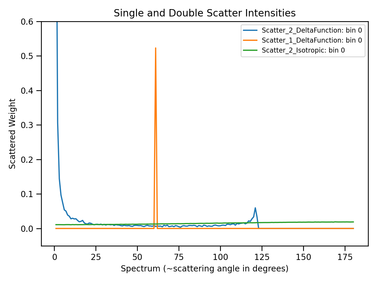
# q=2ksin(theta), so q spike corresonds to single scatter spike at ~60 degrees, double scatter spikes at 0 and 120 degrees
msplot = plotBin('Scatter_2_DeltaFunction',0)
msplot = plotBin('Scatter_1_DeltaFunction',0, window=msplot)
msplot = plotBin('Scatter_2_Isotropic',0, window=msplot)
axes = plt.gca()
axes.set_xlabel('Spectrum (~scattering angle in degrees)')
axes.set_ylim(-0.05,0.6)
plt.title("Single and Double Scatter Intensities")
mtd.clear()

(Source code, png, hires.png, pdf)

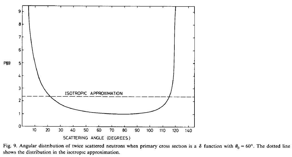
The double scatter profile shows a similar shape to the analytic result calculated in [5]:

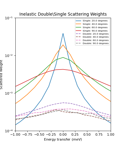
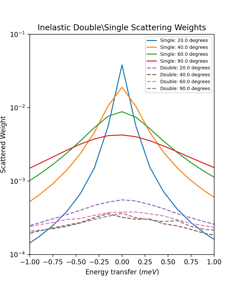
Example - inelastic calculation on direct geometry (matches calculation in DISCUS paper [1] figure 1)

# import mantid algorithms, numpy and matplotlib
from mantid.simpleapi import *
import matplotlib.pyplot as plt
import numpy as np
import math

# parameterised Lorentzian S(Q,w) from Discus pdf
# wavelength = 4 Angstroms, k=1.57
X,Y, SpecAxis =[],[],[]
qmin, qmax = 0.,4.0
nqpts = 9
wmin, wmax = -5.85, 5.85 # meV
nwpts = 79 # negative w is given explicitly so ~double number of pts in Discus
D = 0.15 # Angstom-2 meV -1 = 2.3E-05 cm2 s-1
TEMP=300
HOVERT = 11.6087/TEMP
for iq in range(nqpts):
   q = iq * (qmax-qmin)/(nqpts-1) + qmin
   SpecAxis.append(q)
   for iw in range(nwpts):
     w = iw * (wmax-wmin)/(nwpts-1) + wmin
     X.append(w)
     if (w*w + (D*q*q)**2==0.):
        # Discus S(Q,w) has zero here so do likewise
        print("Denominator zero so outputting S(q,w)=0")
        Y.append(0.)
     else:
        Sqw = D*q*q/(math.pi*(w*w + (D*q*q)**2))
        # Apply detailed balance, neutrons more likely to lose energy in each scatter
        # Mantid has w = Ei-Ef
        if (w > 0.):
           Sqw = Sqw * math.exp(HOVERT * w)
        # S(Q,w) is capped at exactly 4.0 for some reason in Discus example
        Y.append(min(Sqw,4.0))

sqw = CreateWorkspace(DataX=X,DataY=Y,UnitX="DeltaE",
                      VerticalAxisUnit="MomentumTransfer",
                      VerticalAxisValues=SpecAxis, NSpec=nqpts)

two_thetas = [20.0, 40.0, 60.0, 90.0]

ws = CreateSampleWorkspace(WorkspaceType="Histogram",
                           XUnit="DeltaE",
                           Xmin=wmin-0.5*(wmax-wmin)/(nwpts-1),
                           Xmax=wmax+0.5*(wmax-wmin)/(nwpts-1),
                           BinWidth=(wmax-wmin)/(nwpts-1),
                           NumBanks=len(two_thetas),
                           BankPixelWidth=1,
                           InstrumentName="testinst")

# set up ring of detectors in yz plane
ids = list(range(1,len(two_thetas)+1))
EditInstrumentGeometry(ws,
    PrimaryFlightPath=14.0,
    SpectrumIDs=ids,
    L2=[2.0] * len(two_thetas),
    Polar=two_thetas,
    #azimuthal angle=phi, phi=0 along x axis and increases as move towards vertical y axis
    Azimuthal=[-90.0] * len(two_thetas),
    DetectorIDs=ids,
    InstrumentName="testinst")

# flat plate sample 5cm x 5cm x 0.065cm
cuboid_xml = " \
<cuboid id='flatplate'> \
  <width val='0.05' /> \
  <height val='0.05'  /> \
  <depth  val='0.00065' /> \
  <centre x='0.0' y='0.0' z='0.0'  /> \
  <rotate x='45' y='0' z='0' /> \
</cuboid> \
"
SetSample(InputWorkspace=ws,
          Geometry={'Shape': 'CSG', 'Value': cuboid_xml},
          Material={'NumberDensity': 0.02, 'AttenuationXSection': 0.0,
                    'CoherentXSection': 0.0, 'IncoherentXSection': 0.0, 'ScatteringXSection': 80.0})

#match Ei value from DISCUS pdf Figure 1
ws.run().addProperty("deltaE-mode", "Direct", True);
ws.run().addProperty("Ei", 5.1, True);

DiscusMultipleScatteringCorrection(InputWorkspace=ws, StructureFactorWorkspace=sqw,
                                   OutputWorkspace="MuscatResults", NeutronPathsSingle=200,
                                   NeutronPathsMultiple=1000)

# reverse w axis because Discus w = Ef-Ei (opposite to Mantid)
for i in range(mtd['MuscatResults_Scatter_1'].getNumberHistograms()):
    y = np.flip(mtd['MuscatResults_Scatter_1'].dataY(i),0)
    e = np.flip(mtd['MuscatResults_Scatter_1'].dataE(i),0)
    mtd['MuscatResults_Scatter_1'].setY(i,y.tolist())
    mtd['MuscatResults_Scatter_1'].setE(i,e)
for i in range(mtd['MuscatResults_Scatter_2'].getNumberHistograms()):
    y = np.flip(mtd['MuscatResults_Scatter_2'].dataY(i),0)
    e = np.flip(mtd['MuscatResults_Scatter_2'].dataE(i),0)
    mtd['MuscatResults_Scatter_2'].setY(i,y.tolist())
    mtd['MuscatResults_Scatter_2'].setE(i,e)

plt.rcParams['figure.figsize'] = (5, 6)
fig, ax = plt.subplots(subplot_kw={'projection':'mantid'})
for i, tt in enumerate(two_thetas):
    ax.plot(mtd['MuscatResults_Scatter_1'], wkspIndex=i, label='Single: ' + str(tt) + ' degrees')
for i, tt in enumerate(two_thetas):
    ax.plot(mtd['MuscatResults_Scatter_2'], wkspIndex=i, label='Double: ' + str(tt) + ' degrees', linestyle='--')
plt.yscale('log')
ax.set_xlim(-1,1)
ax.set_ylim(1e-4,1e-1)
ax.legend(fontsize=7.0)
plt.title("Inelastic Double\\Single Scattering Weights")
fig.show()
mtd.clear()

(Source code, png, hires.png, pdf)

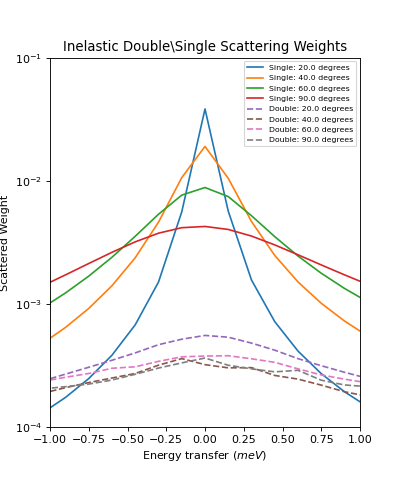
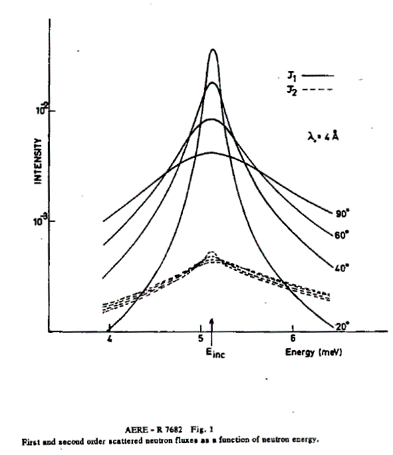
This is the equivalent plot from the original Discus Fortran program:

References

[1] (1,2)

M W Johnson, 1974 AERE Report R7682, Discus: A computer program for the calculating of multiple scattering effects in inelastic neutron scattering experiments

[2]

WS Howells, V Garcia Sakai, F Demmel, MTF Telling, F Fernandez-Alonso, Feb 2010, MODES manual RAL-TR-2010-006, doi: 10.5286/raltr.2010006

[3]

FORTRAN source code for MUSCAT

[4]

R Mancinelli 2012 J. Phys.: Conf. Ser. 340 012033, Multiple neutron scattering corrections. Some general equations to do fast evaluations doi: 10.1088/1742-6596/340/1/012033

[5]

J Mayers, R Cywinski, 1985 Nuclear Instruments and Methods in Physics Research A241, A Monte Carlo Evaluation Of Analytical Multiple Scattering Corrections For Unpolarised Neutron Scattering And Polarisation Analysis Data doi: 10.1016/0168-9002(85)90607-2

Categories: AlgorithmIndex | CorrectionFunctions

Source

C++ header: DiscusMultipleScatteringCorrection.h

C++ source: DiscusMultipleScatteringCorrection.cpp