\(\renewcommand\AA{\unicode{x212B}}\)

HB2AReduce v1

Summary

Performs data reduction for HB-2A POWDER at HFIR

Properties

Name	Direction	Type	Default	Description
Filename	Input	list of str lists		Data files to load. Allowed extensions: [‘.dat’]
IPTS	Input	number	Optional	IPTS number to load from
Exp	Input	number	Optional	Experiment number to load from
ScanNumbers	Input	int list		Scan numbers to load
Vanadium	Input	string		Vanadium file, can be either the vanadium scan file or the reduced vcorr file. If not provided the vcorr file adjacent to the data file will be used. Allowed extensions: [‘.dat’, ‘.txt’]
Normalise	Input	boolean	True	If False vanadium normalisation will not be performed
ExcludeDetectors	Input	int list		Detectors to exclude. If not provided the HB2A_exp???__exclude_detectors.txt adjacent to the data file will be used if it exist
DefX	Input	string		By default the def_x (x-axis) from the file will be used, it can be overridden by setting it here
IndividualDetectors	Input	boolean	False	If True the workspace will include each anode as a separate spectrum, useful for debugging issues
BinData	Input	boolean	True	Data will be binned using BinWidth. If False then all data will be unbinned
BinWidth	Input	number	0.05	Bin size of the output workspace
Scale	Input	number	1	The output will be scaled by this value
OutputWorkspace	Output	Workspace	Mandatory	Output Workspace
SaveData	Input	boolean	True	By default saving the reduced data to either GSAS or XYE
OutputFormat	Input	string	GSAS	Supportted output format: XYE (.dat), GSAS (.gss). Allowed values: [‘XYE’, ‘GSAS’]
OutputDirectory	Input	string		Saving directory for output file

Description

This algorithm reduces HFIR POWDER (HB-2A) data.

You can either specify the filenames of data you want to reduce or provide the IPTS, exp and scan number. If only one experiment exists in an IPTS then exp can be omitted. e.g. the following are equivalent:

ws = HB2AReduce('/HFIR/HB2A/IPTS-21073/exp666/Datafiles/HB2A_exp0666_scan0024.dat')
# and
ws = HB2AReduce(IPTS=21073, exp=666, ScanNumbers=24)

You can specify any number of filenames or scan numbers (in a comma separated list).

Two ways for normalizing reduced data are provided, namely with monitor counts and collection time. The default one would be with monitor count, meaning the value specified with OutputWorkspace parameter would be used as the name of the generated workspace and stem name of output file (if specified) with monitor counts normalization. Along with that, an alternative workspace and corresponding output file would be generated, with ‘_norm_time’ appended to the specified name.

Vanadium

By default the correct vcorr file (HB2A_exp???__Ge_[113|115]_[IN|OUT]_vcorr.txt) adjacent to the data file will be used. Alternatively either the vcorr file or a vanadium scan file can be provided to the Vanadium option. If a vanadium scan file is provided then the vanadium counts can be taken into account when calculating the uncertainty which can not be done with using the vcorr file.

If Normalise=False then no normalisation will be performed.

ExcludeDetectors

By default the file HB2A_exp???__exclude_detectors.txt adjacent to the data file will be used unless a list of detectors to exclude are provided by ExcludeDetectors

IndividualDetectors

If this option is True then a separate spectra will be created in the output workspace for every anode. This allows you to compare adjacent anodes.

Binning Data

If BinData=True (default) then the data will be binned on a regular grid with a width of BinWidth. The output can be scaled by an arbitrary amount by setting Scale.

def_x

This algorithm will read the def_x value in the data file and use it as the x-axis. This value can be overridden by setting the DefX property, e.g. DefX='2theta'.

If you did a scan using a particular anode vs temperature then you should set IndividualDetectors=True and specify DefX if not correct in the data file. Then simply plot the spectrum you are scanning, look at the example below Anode8 vs temperature.

Saving reduced data

The output workspace can be saved to XYE, Maud and TOPAS format using SaveFocusedXYE. e.g.

# XYE with no header
SaveFocusedXYE(ws, Filename='data.xye', SplitFiles=False, IncludeHeader=False)

# TOPAS format
SaveFocusedXYE(ws, Filename='data.xye', SplitFiles=False, Format='TOPAS')

# Maud format
SaveFocusedXYE(ws, Filename='data.xye', SplitFiles=False, Format='MAUD')

You can also save the reduced data as GSAS or XYE format by adding additional arguments to the reduction call

ws = HB2AReduce(
   '/HFIR/HB2A/IPTS-21073/exp666/Datafiles/HB2A_exp0666_scan0024.dat',
   SaveData=True,
   OutputFormat="GSAS",
   OutputDirectory="/tmp",
   )

Warning - Do not specify OutputFormat or OutputDirectory if SaveData is set to False. - If def_x = 2theta is not the in the header of any one of the input files, do not set OutputFormat to GSAS.

Usage

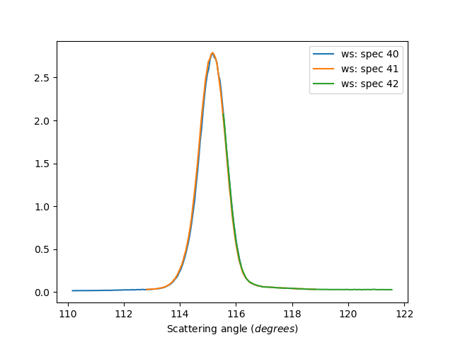
Individual Detectors

ws=HB2AReduce('HB2A_exp0666_scan0024.dat', IndividualDetectors=True)

# Plot anodes 40, 41 and 42
import matplotlib.pyplot as plt
from mantid import plots
fig, ax = plt.subplots(subplot_kw={'projection':'mantid'})
for num in [40,41,42]:
    ax.plot(ws, specNum=num)
plt.legend()
#fig.savefig('HB2AReduce_1.png')
plt.show()

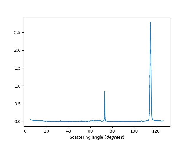
Unbinned data

ws=HB2AReduce('HB2A_exp0666_scan0024.dat', BinData=False)

# Plot
import matplotlib.pyplot as plt
from mantid import plots
fig, ax = plt.subplots(subplot_kw={'projection':'mantid'})
ax.plot(ws)
#fig.savefig('HB2AReduce_2.png')
plt.show()

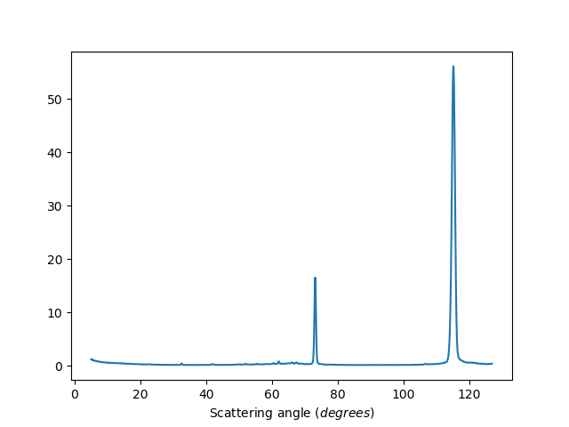
Binned data

ws=HB2AReduce('HB2A_exp0666_scan0024.dat')

# Plot
import matplotlib.pyplot as plt
from mantid import plots
fig, ax = plt.subplots(subplot_kw={'projection':'mantid'})
ax.plot(ws)
#fig.savefig('HB2AReduce_3.png')
plt.show()

Exclude detectors: 1-20,40,41,42

ws=HB2AReduce('HB2A_exp0666_scan0024.dat', ExcludeDetectors='1-20,40,41,42')

# Plot
import matplotlib.pyplot as plt
from mantid import plots
fig, ax = plt.subplots(subplot_kw={'projection':'mantid'})
ax.plot(ws)
#fig.savefig('HB2AReduce_4.png')
plt.show()

Combining multiple files

ws=HB2AReduce('HB2A_exp0666_scan0024.dat, HB2A_exp0666_scan0025.dat')

# Plot
import matplotlib.pyplot as plt
from mantid import plots
fig, ax = plt.subplots(subplot_kw={'projection':'mantid'})
ax.plot(ws)
#fig.savefig('HB2AReduce_5.png')
plt.show()

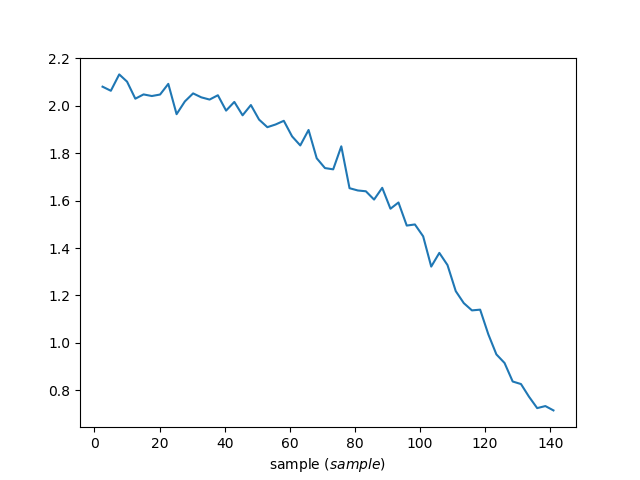
Anode8 vs temperature

Because the following data file has def_x = sample then this algorithm will reduce the data to be counts vs sample (sample temperature). Setting IndividualDetectors=True allows you to see a single anode vs temperature.

ws=HB2AReduce('HB2A_exp0660_scan0146.dat',
              Vanadium='HB2A_exp0644_scan0018.dat',
              IndividualDetectors=True)

# Plot
import matplotlib.pyplot as plt
from mantid import plots
fig, ax = plt.subplots(subplot_kw={'projection':'mantid'})
ax.plot(ws, specNum=8) # anode8
#fig.savefig('HB2AReduce_6.png')
plt.show()

Categories: AlgorithmIndex | Diffraction\Reduction

Source

Python: HB2AReduce.py