\(\renewcommand\AA{\unicode{x212B}}\)

The Basics of Data Reduction

This section explains:

• the concept of t_zero and t_good

• the concept of dead time correction

• how to set the detector calibration factor, \({\alpha}\)

• how to group data

The concept of t_zero and t_good

Since the muon data collected at ISIS is pulsed, the analysis of data produced by the equipment must account for this. The concept of t_zero and t_good and is what is used to determine the start of a good pulsed data set.

The timing origin, t_zero, for the muon response in the sample is when the middle of the muon pulse has reached the sample.

However, the good data region is not obtained until the entire pulse has arrived at the sample, this time is defined as t_good.

The difference between t_good and t_zero is t_{good offset}.

When using the Muon Analysis GUI, t_zero and t_good are loaded from the NeXuS file (having been determined by the instrument scientist).

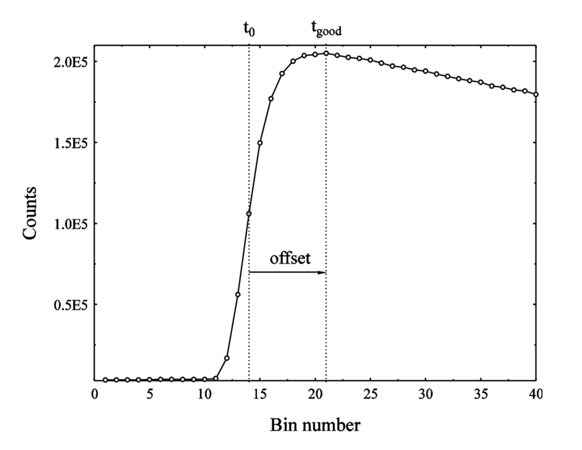
Figure 13: A diagram showing t_zero, t_good and t_{good offset} at a muon pulse.

The concept of dead-time

After a detector has recorded a positron count there is a small time interval before it is able to detect another count. It is possible, especially at the high data collection rates now available on the muon instruments, that a positron will arrive within this interval and not be recorded. Statistical analysis can be used to correct for this. A silver sample is used to determine dead time values for each detector, the results of which are made into a dead time data file. The NeXuS format stores this data internally. For further information about the correction of detector deadtime see: Kilcoyne, RAL report RAL-94-080 (1994).

To observe the effect of dead time, follow the instructions below:

1. Open the Muon Analysis GUI and make sure ‘none’ is selected for Dead Time Correction (in the Instrument section of the Home Tab)

2. Load data file EMU00034998.nxs using the GUI.

3. This example is best viewed with a fixed rebin with steps of ten, select Fixed from the dropdown menu and then type 10 into the box.

4. A simple way to compare this data to some with dead time correction is to change the name so that Mantid does not automatically update the workspace. Go to the workspaces pane and navigate via EMU34998 > EMU34998 Pairs, and right click on the Rebin dataset, then select Rename and pick a suitable new name such as NoDeadTime, then click on Run.

5. Plot this data as described by Loading Data in Other Mantid Functions and Basic Data Manipulation.

6. The effect of the dead time correction is most apparent in the first 16 \({\mu s}\), to easily view this portion of the data, use the Figure Options to set the plot’s the X-Axis limits to 0-16 \({\mu s}\), and Y-Axis limits to 0.158-0.176. How to do this is given in the Overlaying Data and Changing Plot Style section of Other Mantid Functions and Basic Data Manipulation.

7. Reopen the Mantid Muon GUI and change the setting of the Dead Time Correction drop-down menu from None to from data file.

8. Return to the EMU34998 Pairs workspace as in step 4. There should now be a new Rebin dataset along with the renamed one, Overplot this new spectrum onto the plot of NoDeadTime. (see Overlaying Data and Changing Plot Style section of Other Mantid Functions and Basic Data Manipulation for this process). Consider the differences between the two curves.

Figure 14: The effect of dead time correction on a data set.

The detector calibration factor, Alpha

The detector calibration factor, α, used to normalise the asymmetry, can be determined by the use of the Guess Alpha tool on any detector group pairing. By default, using the asymmetry equation shown below, the α value is approximated to be 1. However, the Guess Alpha tool allows for a more accurate determination of the α value for a particular data set.

As an exercise, follow the instructions below to guess an \({\alpha}\) value and observe the resulting changes.

1. Using the GUI, load a transverse field measurement, such as MUSR00024563.

2. Select the Grouping tab

Note that when a data file is loaded using the GUI, the default option for the MuSR spectrometer is to GROUP (or add) all data in detectors 1-32 (a group of detectors referred to as bck) together. Similarly, data in detectors 33-64 (a group called fwd) is summed.

3. To generate \({\alpha}\) click on Guess Alpha. This process is shown in Figure 15.

Figure 15: How to use the Guess Alpha tool in the Muon Analysis GUI.

What has happened? (reloading the data file might be needed to observe the changes.)

4. Try creating a pair called sample_long as described in The Tabs - Grouping and using Guess Alpha with this group highlighted rather than long. Consider the changes that can be observed.