Table of Contents
| Name | Direction | Type | Default | Description |
|---|---|---|---|---|
| SampleWorkspace | Input | MatrixWorkspace | Mandatory | Name for the input Sample workspace. |
| CorrectionsWorkspace | Input | WorkspaceGroup | Name for the input Corrections workspace. | |
| CanWorkspace | Input | MatrixWorkspace | Name for the input Can workspace. | |
| CanScaleFactor | Input | number | 1 | Factor to scale the can data |
| OutputWorkspace | Output | MatrixWorkspace | Mandatory | The output corrections workspace. |
Applies absorption corrections calculated in the Paalman & Pings absorption
factor format:  (correction factor for scattering and absorption
in sample),
  (scattering in sample and absorption in sample and
container),
  (scattering in container and absorption in sample
and container) and
  (scattering and absorption in container).
This algorithm can be used to apply absorption corrections calculated with either the CylinderPaalmanPingsCorrection v2 and FlatPlatePaalmanPingsCorrection v1 algorithms as well as the legacy indirect calculate correcteions routine, providing that the sample and container are first converted to wavelength and the corrections are interpolated to match the sample as demonstrated in the example below.
Depending on the input workspaces provided to the algorithm it may operate in one of three ways, each of which is described on a separate workflow diagram.
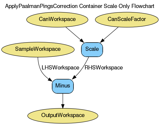
In the case where only a container workspace and no correction factors are provided.

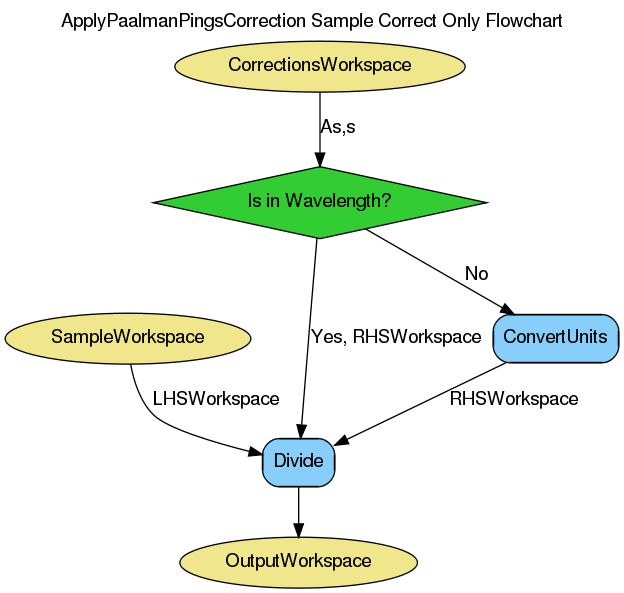
In the case where only correction factors and no container workspace is provided.

Example: using with legacy indirect corrections data
# Load the sample and can
sample_ws = Load('irs26176_graphite002_red.nxs')
can_ws = Load('irs26173_graphite002_red.nxs')

# Convert sample and container workspaces to wavelength
sample_ws = ConvertUnits(InputWorkspace=sample_ws,
                         Target='Wavelength',
                         EMode='Indirect',
                         EFixed=1.845)
can_ws = ConvertUnits(InputWorkspace=can_ws,
                      Target='Wavelength',
                      EMode='Indirect',
                      EFixed=1.845)

# Load the corrections workspace
corrections_ws = Load('irs26176_graphite002_cyl_Abs.nxs')

# Interpolate each of the correction factor workspaces to match the
# binning of the smaple
# Required to use corrections from the old indirect calculate
# corrections routines
for factor_ws in corrections_ws:
    SplineInterpolation(WorkspaceToMatch=sample_ws,
                        WorkspaceToInterpolate=factor_ws,
                        OutputWorkspace=factor_ws,
                        OutputWorkspaceDeriv='')

corr = ApplyPaalmanPingsCorrection(SampleWorkspace=sample_ws,
                                   CorrectionsWorkspace=corrections_ws,
                                   CanWorkspace=can_ws)

print 'Corrected workspace has %d spectra over %d bins' % (
      corr.getNumberHistograms(), corr.blocksize())

print 'Type of correction applied: %s' % (
      corr.getRun()['corrections_type'].value)
Output:
Corrected workspace has 10 spectra over 1905 bins
Type of correction applied: sample_and_can_corrections
Categories: Algorithms | Workflow | MIDAS | PythonAlgorithms