Table of Contents
This interface aims at integrating and simplifying the following tasks related to tomographic reconstruction and imaging with neutrons. While much of its functionality is being developed in a generic way, it is presently being tested and trialed for the IMAT instrument at ISIS.
An important feature of this interface is the capability to submit jobs to a remote compute resource (a compute cluster for example). Currently remote jobs are run on the SCARF cluster, administered by the Scientific Computing Department of STFC. You can also use this cluster via remote login and through its web portal. This resource is available for ISIS users.
Warning
This interface is undergoing heavy works. The sections or tabs are subject to changes and reorganization.New functionality is being added and the pre-post-processing and reconstruction workflow is being modified based on feedback from initial test data.
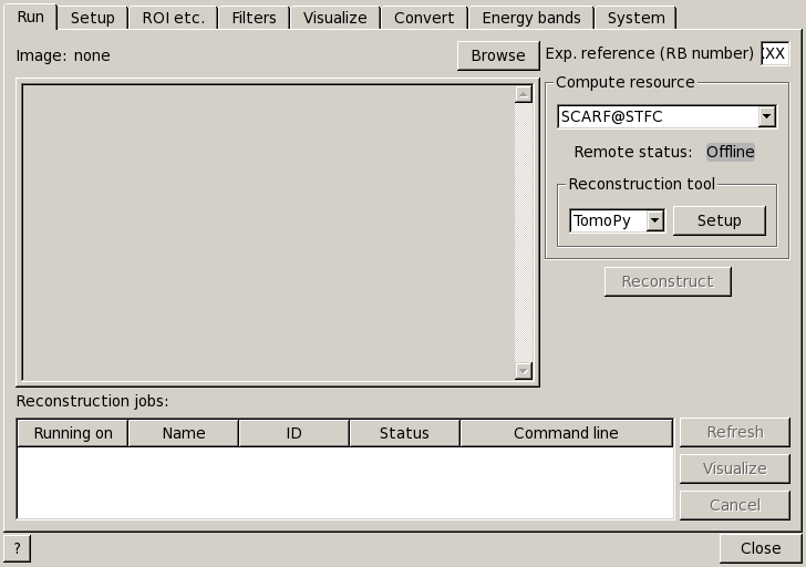
By default the interface shows the Run tab, where you can visualize images, submit reconstruction jobs, see and control the status of the jobs submitted recently.
In the setup tab you can set the details of the remote and/or local compute resources. Importantly, here is where you can set you username and password to log into the remote compute resource. To be able to run jobs remotely you first need to log into the remote compute resource. Once you log in, an automatic mechanism will periodically query the status of jobs (for example every minute). You can also update it at any time by clicking on the refresh button.
In this tab you also have to set the folders/directories where the input data for reconstruction jobs is found. This information is required every time you start analyzing a new dataset. The required fields are:

NB: This interface is under heavy development. Several practical details lack polishing and/or are missing. This implies that there may be usability issues at times and some steps may not be as intuitive or simple as they could. Please, do not hesitate to provide suggestions and feedback.
The next sections provide further details that might be needed to fully understand the process of generating tomographic reconstructions with this interface.
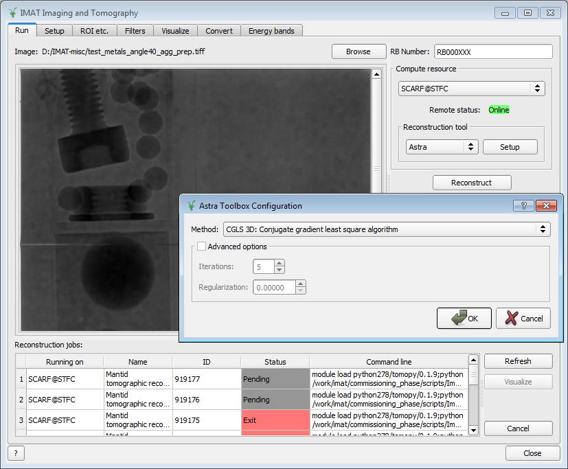
At the moment two reconstruction tools are being set up and trialed on SCARF and some ISIS machines:
References for the Astra Toolbox:
References for TomoPy:
In the near future it is expected that support will be added for Savu: Tomography Reconstruction Pipeline, developed at the Diamond Light Source.
References for Savu:
In principle, users do not need to deal with specificities of different file formats. That is the aim of this interface, but as it is currently being developed, and for reference a brief list of relevant file and data formats is given here:
These formats are used in different processing steps and parts of this interface. For example, you can visualize FITS and TIFF images in the Run tab and also in the ROI, etc. tab. As another example, the reconstruction tools typically need as inputs at least a stack of images which can be in different formats, including a set of FITS or TIFF files, or a single DLS NXTomo file. Other third party tools use files in these formats as inputs, outputs or both.
This is dependent on the facility and instrument.
Warning
This is work in progress. At ISIS, in principle data will be replicated in the ISIS archive, the IMAT disk space on the cluster SCARF (remote compute resource), and possibly an IMAT analysis machine.
The path to the files of a particular tomographic reconstruction consists of several components. An example path would be (on a Windows system where the input/output data is on the drive “D”:
where:
As the files are mirrored on the remote computer cluster, if a network drive have been added (or mapped) in the local system, for example using the drive “S:”, then the following path would contain a similar tree of image files:
The equivalent on a non-Windows system would be for example:
These and related parameters can be inspected and modified in the sytem settings section (or System tab). Their default values are set for the current setup of the IMAT analysis machine. The “Reset all” button resets all these settings to their factory defaults. Note that the System section of the interface is currently work in progress and it may change significantly as required during commissioning of IMAT.
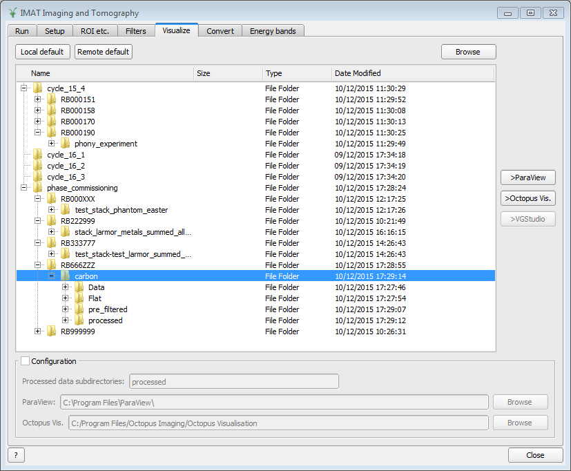
The tab Visualization has simple push buttons to browse the files available from the local and remote locations, as well as any other directory or folder selected by the user. The data for the different experiments can be found under these locations.
To be able to run jobs on a remote compute resource (cluster, supercomputer, etc.)
You can monitor the status of the jobs currently running (and recently run) on remote compute resources in the same tab.
Before any reconstruction job is started several pre-/post-processing options would normally need to be fine tuned for the sample data to be processed correctly. The region of interest and the “air” region (or region for normalization) can be set visually in a specific tab. All other pre- and post-processing settings are defined in a separate tab.
Several parameters can be set in the ROI etc. section or tab. These parameters will be used for all the reconstruction jobs, regardless of the tool and/or reconstruction method used.

Stacks of images can be opened by using the browse button located at the top of the interface. You can point the interface to a folder (directory) containing directories for sample, dark, and flat images, or alternatively to a folder containing images. The interface will pick all the files recognized as images.
At any stage during the process of selecting the regions it is also possible to see how the selections fit different images by sliding through the images of the stack (using the slider or scroll bar).
The center of rotation can be selected interactively by clicking on the select button and then clicking on an image pixel. To select the regions of interest or the area of normalization, just click on the respective “select” button and then click and drag with the mouse to select a rectangle. The precise coordinates of the center and regions can be set via the boxes of the right panel as well.
Once you have selected or set one of the regions, or the center, they can be selected again by pushing the respective “Select” buttons and/or editing their coordinates manually.
The default values, set in principle when a new stack of images is loaded, are as follows. The region of intererest is set to cover all the images. The regions of normalization is not set (empty), and the center of rotation is set to the center of the image. The option to find the center of rotation automatically is disabled at present.
If when selection a region the mouse is moved outside of the images, it is possible to continue the selection of the region (second corner) by clicking again inside the image. Alternatively, any selection can be reset at any point by using the “reset” buttons.
When loading a stack of images, note that when the images are loaded from the folder(s) (directorie(s)) any files with unrecognized extension or type (for example .txt) will be ignored. Normally a warning about this will be shown in the Mantid logs. Image files with the string _SummedImg at the end of their names will be skipped as well, as this is a convention used by some detectors/control software to generate summed images
The Filters tab can be used to set up the pre- and post-processing steps. These are applied regardless of the particular tomographic reconstruction tool and algorithm used when running reconstruction jobs. Pre-processing filters are applied on the raw input images before the reconstruction algorithm is run. Post-processing steps are applied on the reconstructed volume produced by the algorithm.

Among other options, normalization by flat and/or dark images can be enabled here. Note that this setting is global and will be effective for any input dataset. In the Setup section it is possible to enable or disable them specifically for the dataset being processed.
The tab also shows options to define what outputs should be produced in addition to the reconstructed volume.
The settings are remembered between sessions. It is possible to reset all the settings to their original defaults by clicking on the reset button.
The results are written into the output paths selected in the interface (in the setup section or tab). For every reconstructed volume a sequence of images (slices along the vertical axis) are written. In addition, two complementary outputs are generated in the same location:
This capability is being developed at the moment, and it requires additional setup steps on the local analysis machine. Basic functionality is supported only on the IMAT data analysis machine.
Warning
The interface is being extended to have integration with third party tools for 3D visualization and segmentation. This is work in progress.
The Visualization tab can be used to browse the local and remote locations where results are stored. It is also possible to open these results in third party visualization applications. NB: ParaView is currently supported and additional tools are being integrated.
Warning
The interface is being extended to provide different methods of combining energy bands from energy selective experiments. This is work in progress.
Here it is possible to aggregate stacks of images normally acquired as energy/wavelength selective data. This interface is based on the algorithm ImggAggregateWavelengths which supports different ways of aggregating the input images. In the simplest case, a number of output bands can be produced by aggregating the input bands split into uniform segments. This is called “uniform bands”. When the number of uniform bands is one, all the wavelengths are aggregated into a single output stack. It is also possible to specify a list of boundaries or ranges of image indices. For example if an input dataset consists of 1000 images per projection angle (here indexed from 0 to 999), three partially (50%) overlapping output bands could by produced by specifying the ranges as “0-499, 250-749, 500-999”. In principle it is also possible to aggregate images by time of flight ranges, based on specific extension headers that must be included in the input (FITS) images. This option is disabled at the moment. Please refer to the documentation of ImggAggregateWavelengths for lower level details on how the algorithm processes the input directories and files.


This interface provides a simple way of converting stacks of images between diferent formats. This is for convenience and interoperability with third party tools that for example may not be able to load FITS images but require them in TIFF format. All the images found under the input path (directory) will be converted from the input format selected into the output format. The output images will be created under the output path (directory) with the same tree structure as the input images.
The conversion process will look for images recursively inside the input directory. That is, it will process all its subdirectories and the subdirectories of these up to a given maximum depth. To limit the search depth. The usual default value is 3 which is sufficient for stacks of images and sets of stacks of images from a series of samples for an experiment, following the conventions for IMAT tomography data. If higher depth values than the default are used we recommend to take extreme care, making sure the input path given makes sense. This process can be lengthy and demanding in terms of disk space when processing more than one or a small number of experiments (RB reference numbers), and especially so for wavelength dependent experiments.
TODO: how to use it. Hints.
TODO: how to use it. Hints.
Savu uses a specific file format developed by the Diamond Light Source, the DLS NXTomo. A few examples can be found from the savu repository on GitHub.
A Savu reconstruction pipeline is defined by a list of processing steps (or plugins) and their parameters. In the Savu setup dialog this list is built on the right panel (current configuration) by adding and sorting available plugins available from the tree shown on the left panel. From the file menu, different savu configurations can be saved for later use and loaded from previously saved files.
Categories: Interfaces | Diffraction