\(\renewcommand\AA{\unicode{x212B}}\)

Data reduction for D7 instrument at the ILL¶

Table of contents

There are three workflow algorithms supporting data reduction at ILL’s D7 polarised diffraction and spectroscopy instrument. These algorithms are:

D7YIGPositionCalibration v1: Performs wavelength and position calibraiton for D7 instrument banks and individual detectors in banks.
PolDiffILLReduction v1: Performs data reduction and produces the unnormalised sample cross-sections in one of the available units.
D7AbsoluteCrossSections v1: Performs cross-section separation into nuclear coherent, spin-incoherent and magnetic components, and does the data normalisation.

Together with the other algorithms and services provided by the Mantid framework, the reduction algorithms can handle a number of reduction scenarios. If this proves insufficient, however, the algorithms can be accessed using Python. Before making modifications it is recommended to copy the source files and rename the algorithms as not to break the original behavior.

This document tries to give an overview on how the algorithms work together via Python examples. Please refer to the algorithm documentation for details of each individual algorithm.

Reduction workflow and recommendations ¶

A description of the usage of the algorithms for the D7 data reduction is presented along with several possible workflows, depending on the number of desired corrections and the type of normalisation.

Reduction basics ¶

Note

To run these usage examples please first download the usage data, and add these to your path. In Mantid this is done using Manage User Directories.

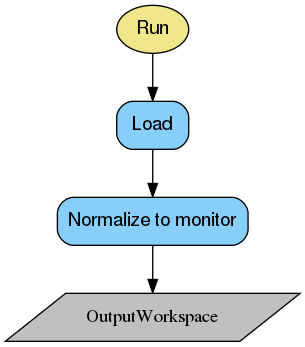
A very basic reduction would include a vanadium reference and a sample, without any corrections or position and wavelength calibration, and follow the steps:

Reduce vanadium data.
Reduce sample data.
Run normalisation with vanadium reduction output as input.

# Define vanadium properties:
vanadiumProperties = {'FormulaUnits': 1, 'SampleMass': 8.54, 'FormulaUnitMass': 50.94}

# Vanadium reduction
PolDiffILLReduction(Run='396993', ProcessAs='Vanadium', OutputTreatment='Sum',
                    OutputWorkspace='reduced_vanadium',
                    SampleAndEnvironmentProperties=vanadiumProperties)

# Define the number of formula units for the sample
sampleProperties = {'FormulaUnits': 1, 'SampleMass': 2.932, 'FormulaUnitMass': 182.54}
# Sample reduction
PolDiffILLReduction(Run='397004', ProcessAs='Sample', OutputWorkspace='reduced_sample',
                        SampleAndEnvironmentProperties=sampleProperties)

# normalise sample and set the output to absolute units with vanadium
D7AbsoluteCrossSections(InputWorkspace='reduced_sample', OutputWorkspace='normalised_sample',
                        SampleAndEnvironmentProperties=sampleProperties,
                        NormalisationMethod='Vanadium', VanadiumInputWorkspace='reduced_vanadium')

SofQ = mtd['normalised_sample']
xAxis = SofQ[0].readX(0)  # TwoTheta axis
print('dS/dOmega (TwoTheta) detector position range: {:.2f}...{:.2f} (degrees)'.format(xAxis[0], xAxis[-1]))

Output:

dS/dOmega (TwoTheta) detector position range: 13.14...144.06 (degrees)

Wavelength and position calibration ¶

The first step of working with D7 data is to ensure that there exist a proper calibration of the wavelength, bank positions, and detector positions relative to their bank. This calibration can be either taken from a previous experiment performed in comparable conditions or obtained from the \(\text{Y}_{3}\text{Fe}_{5}\text{O}_{12}\) (YIG) scan data using a dedicated algorithm D7YIGPositionCalibration. The method follows the description presented in Ref. [1].

This algorithm performs wavelength and position calibration for both individual detectors and detector banks using measurement of a sample of powdered YIG. This data is fitted with Gaussian distributions at the expected peak positions. The output is an Instrument Parameter File readable by the LoadILLPolarizedDiffraction algorithm that will place the detector banks and detectors using the output of this algorithm.

The provided YIG d-spacing values are loaded from an XML list. The default d-spacing distribution for YIG available in Mantid in D7_YIG_peaks.xml file is coming from Ref. [2]. As long as this d-spacing list is sufficient and does not require changes, the YIGPeaksFile property does not need to be specified. The peak positions are converted into \(2\theta\) positions using the initial assumption of the neutron wavelength. YIG peaks in the detector’s scan are fitted separately using a Gaussian distribution.

The workspace containing the peak fitting results is then fitted using a Multidomain function of the form:

\[2\theta_{\text{fit}} = m \cdot (2.0 \cdot \text{asin} ( \lambda / 2d ) + offset_{\text{pixel}} + offset_{\text{bank}}),\]

where m is the bank slope, \(offset_{\text{pixel}}\) is the relative offset to the initial assumption of the position inside the detector bank, and \(offset_{\text{bank}}\) is the offset of the entire bank. This function allows to extract the information about the wavelength, detector bank slopes and offsets, and the distribution of detector offsets.

It is strongly advised to first run the D7YIGPositionCalibration algorithm with the FittingMethod set to None, so that the initial guesses for the positions of the YIG Bragg peaks can be inspected and corrected if needed. Assuming the first python code-block below is used for this purpose, the workspace name to use for inspection of the initial guesses is named peak_fits_fitting_test. There, the initial guesses for individual detectors can be checked against the measured YIG Bragg peaks distribution. The correction can be done by changing the bank offsets, changing the desired peaks width and the minimal distance between them.

To save time in this iterative process, InputWorkspace property can be specified instead of Filenames. This way, the 2D distribution of measured intensities does not have to be created each time from loaded data but can be cached and reused for time saving. To profit from this feature, comment the Filenames property and uncomment the InputWorkspace in the first example below.

Example - D7YIGPositionCalibration - initial guess check before fitting at the shortest wavelength

approximate_wavelength = '3.1' # Angstrom
D7YIGPositionCalibration(
             Filenames='402652:403041',
#            InputWorkspace='conjoined_input_fitting_test',
             ApproximateWavelength=approximate_wavelength,
             YIGPeaksFile='D7_YIG_peaks.xml',
             MinimalDistanceBetweenPeaks=1.5,
             BraggPeakWidth=1.5,
             BankOffsets=[0,0,0],
             MaskedBinsRange=[-50, -25, 15],
             FittingMethod='None',
             ClearCache=False,
             FitOutputWorkspace='fitting_test')

Example - D7YIGPositionCalibration - calibration at the shortest wavelength

approximate_wavelength = '3.1' # Angstrom
D7YIGPositionCalibration(Filenames='402652:403041', ApproximateWavelength=approximate_wavelength,
                            YIGPeaksFile='D7_YIG_peaks.xml', CalibrationOutputFile='test_shortWavelength.xml',
                            MinimalDistanceBetweenPeaks=1.5, BankOffsets=[3,3,-1],
                            MaskedBinsRange=[-50, -25, 15], FittingMethod='Global', ClearCache=True,
                            FitOutputWorkspace='shortWavelength')

print('The calibrated wavelength is: {0:.2f}'.format(float(approximate_wavelength)*mtd['shortWavelength'].column(1)[1]))
print('The bank2 gradient is: {0:.3f}'.format(1.0 / mtd['shortWavelength'].column(1)[0]))
print('The bank3 gradient is: {0:.3f}'.format(1.0 / mtd['shortWavelength'].column(1)[176]))
print('The bank4 gradient is: {0:.3f}'.format(1.0 / mtd['shortWavelength'].column(1)[352]))

Transmission calculation ¶

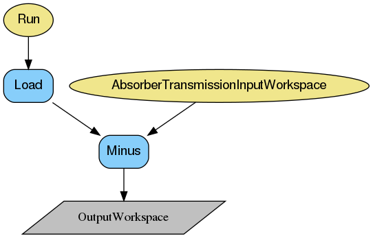
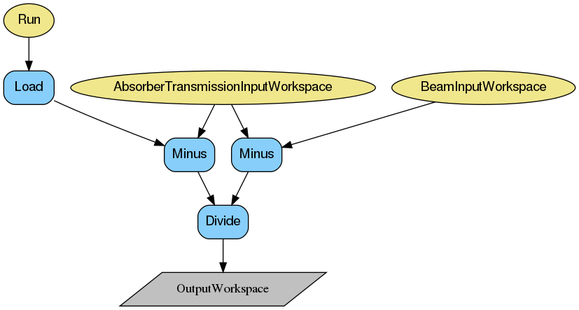
The transmission (T) is calculated using counts measured by monitor 2 (M2), and according to the following formula:

\[T = \frac{S - E_{Cd}}{E - E_{Cd}},\]

where \(S\) is M2 counts measured with the current sample, \(E_{Cd}\) is counts when cadmium absorber is measured, and \(E\) is counts from the direct beam.

The measurement of the cadmium absorber is optional and does not have to be provided as input for the transmission to be calculated. However, it allows to take into account dark currents in the readout system electronics and thus this measurement is advised to be included in transmission calculations.

It is possible to provide more than one numor as input for the transmission calculation. In such a case, the input workspaces are averaged.

The output of the transmission calculation is given as a WorkspaceGroup with a single workspace containing a single value of the calculated polarisation.

Workflow diagrams and working example ¶

Below are the relevant workflow diagrams describing reduction steps of the transmission calculation.

Absorber ¶

Empty container ¶

../_images/PolDiffILLReduction-v1_beam_wkflw.png

Transmission ¶

Note

To run these usage examples please first download the usage data, and add these to your path. In Mantid this is done using Manage User Directories.

Example - transmission calculation for quartz sample

# Beam with cadmium absorber, used for transmission
PolDiffILLReduction(
    Run='396991',
    OutputWorkspace='cadmium_transmission_ws',
    ProcessAs='BeamWithCadmium'
)
# Beam measurement for transmisison
PolDiffILLReduction(
    Run='396983',
    OutputWorkspace='beam_ws',
    CadmiumTransmissionInputWorkspace='cadmium_transmission_ws_1',
    ProcessAs='EmptyBeam'
)
print('Cadmium absorber transmission is {0:.3f}'.format(mtd['cadmium_transmission_ws_1'].readY(0)[0] / mtd['beam_ws_1'].readY(0)[0]))

# Quartz transmission
PolDiffILLReduction(
    Run='396985',
    OutputWorkspace='quartz_transmission',
    CadmiumTransmissionInputWorkspace='cadmium_transmission_ws_1',
    BeamInputWorkspace='beam_ws_1',
    ProcessAs='Transmission'
)
print('Quartz transmission is {0:.3f}'.format(mtd['quartz_transmission_1'].readY(0)[0]))

Output:

Cadmium absorber transmission is 0.011
Quartz transmission is 0.700

Polarisation correction ¶

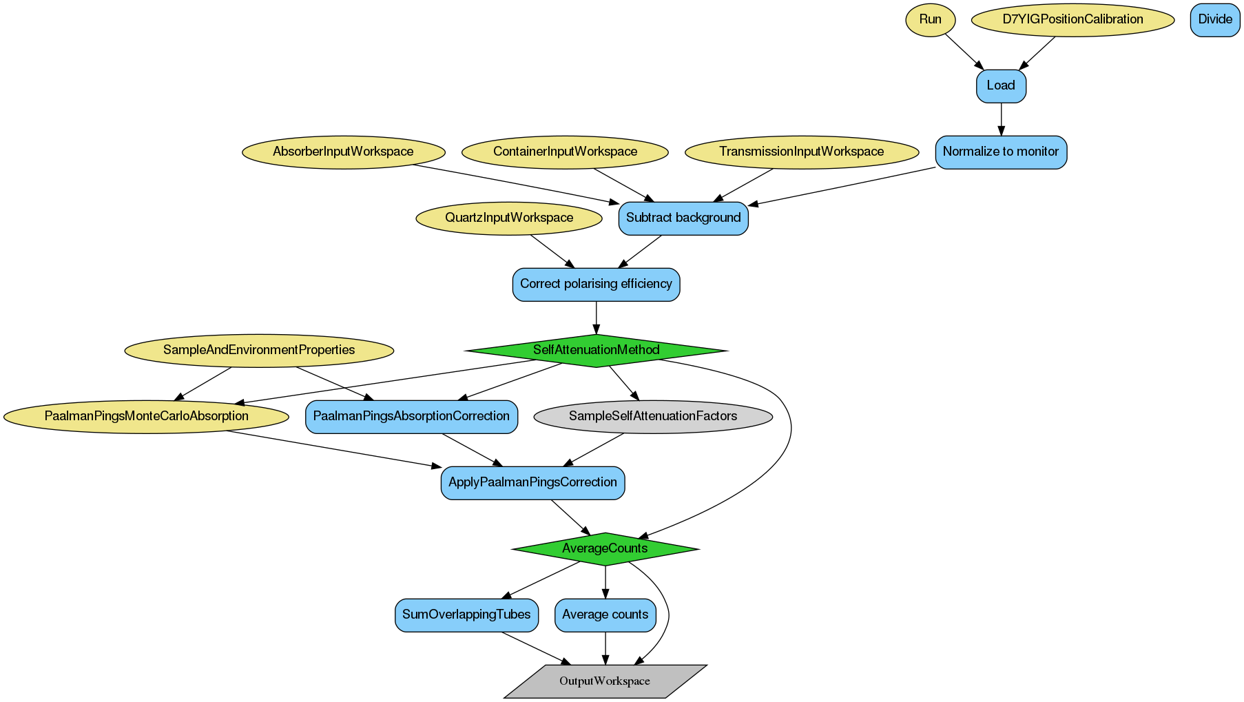
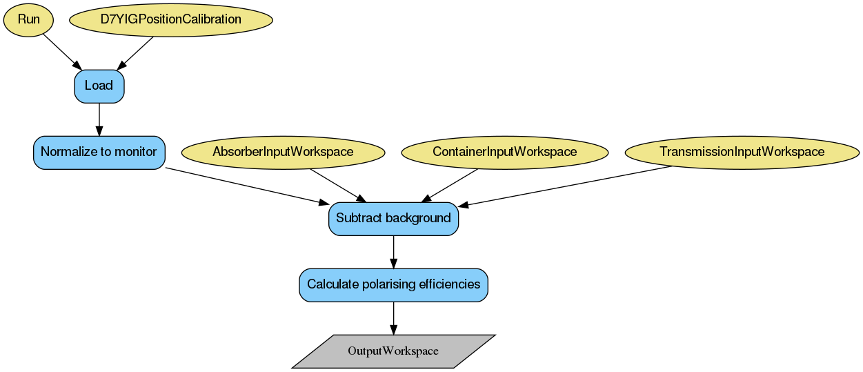
The polarisation correction is estimated using quartz sample. The scattering is purely diffuse and, to a good approximation, non-spin flip. Ideally, the quartz should have the same geometry and attenuation as the sample as then the same gauge volume of the beam is measured and the reduction will give an accurate estimation of the polarizing efficiency. However, the correction is usually fairly insensitive to small differences in the polarizing efficiency and choosing the quartz to have the same outer dimensions is normally satisfactory. Multiple scattering is not a problem, as the correction is given by a ratio and there is no spin-flip scattering to depolarize the beam. The polarization efficiencies are calculated from ratios of non-spin-flip to spin-flip scattering, hence absolute numbers are not necessary.

First, the data is normalised to monitor 1 (M1). Then, if the necessary inputs of empty container and absorber (please note this is a different measurement than mentioned in the Transmission section) measurements are provided, the background can be subtracted from the data:

\[\dot{I_{B}} = \dot{I} - T\dot{E} - (1-T) \dot{C},\]

where \(\dot{I}\) denotes monitor-normalised quartz data, \(T\) is transmission, and \(\dot{E}\) and \(\dot{C}\) are the normalised counts measured with empty container and cadmium absorber, respectively.

In the case where either absorber or empty container inputs are not provided, this correction is not performed.

Finally, the polariser-analyser efficiency can be calculated, using the following formula:

\[\phi = \frac{\dot{I_{B}}(00) - \dot{I_{B}}(01)}{(2f_{p}-1) \dot{I_{B}}(00) + \dot{I_{B}}(01)},\]

where \(f_{p}\) is the flipper efficiency, currently assumed to be 1.0, and \(\dot{I_{B}}(00)\) and \(\dot{I_{B}}(01)\) denote normalised and background-subtracted data with flipper states off and on respectively.

The output is given in as a WorkspaceGroup with the number of entries consistent with the number of measured polarisation directions. Each workspace in the group contains a single value of the polariser-analyser efficiency per detector. The flipping ratios are also available for inspection in a WorkspaceGroup named flipping_ratios.

Workflow diagram and working example ¶

Below is the relevant workflow diagram describing reduction steps of the quartz reduction.

../_images/PolDiffILLReduction-v1_quartz_wkflw.png

Note

To run these usage examples please first download the usage data, and add these to your path. In Mantid this is done using Manage User Directories.

Example - full treatment of a sample

# Beam with cadmium absorber, used for transmission
PolDiffILLReduction(
    Run='396991',
    OutputWorkspace='cadmium_transmission_ws',
    ProcessAs='BeamWithCadmium'
)

# Beam measurement for transmisison
PolDiffILLReduction(
    Run='396983',
    OutputWorkspace='beam_ws',
    CadmiumTransmissionInputWorkspace='cadmium_transmission_ws_1',
    ProcessAs='EmptyBeam'
)

# Quartz transmission
PolDiffILLReduction(
    Run='396985',
    OutputWorkspace='quartz_transmission',
    CadmiumTransmissionInputWorkspace='cadmium_transmission_ws_1',
    BeamInputWorkspace='beam_ws_1',
    ProcessAs='Transmission'
)

# Empty container
PolDiffILLReduction(
    Run='396917',
    OutputWorkspace='empty_ws',
    ProcessAs='Empty'
)

# Absorber
PolDiffILLReduction(
    Run='396928',
    OutputWorkspace='cadmium_ws',
    ProcessAs='Cadmium'
)

# Polarisation correction
PolDiffILLReduction(
    Run='396939',
    OutputWorkspace='pol_corrections',
    CadmiumInputWorkspace='cadmium_ws',
    EmptyInputWorkspace='empty_ws',
    TransmissionInputWorkspace='quartz_transmission_1',
    OutputTreatment='Average',
    ProcessAs='Quartz'
)

SumSpectra(InputWorkspace='pol_corrections_ZPO_0', OutputWorkspace='sum',
           StartWorkspaceIndex=0, EndWorkspaceIndex=131)
print("The average polarisation efficiency in the Z direction is {0:.2f}".format(mtd['sum'].readY(0)[0] / 132.0))

Output:

The average polarisation efficiency in the Z direction is 0.90

Vanadium data reduction ¶

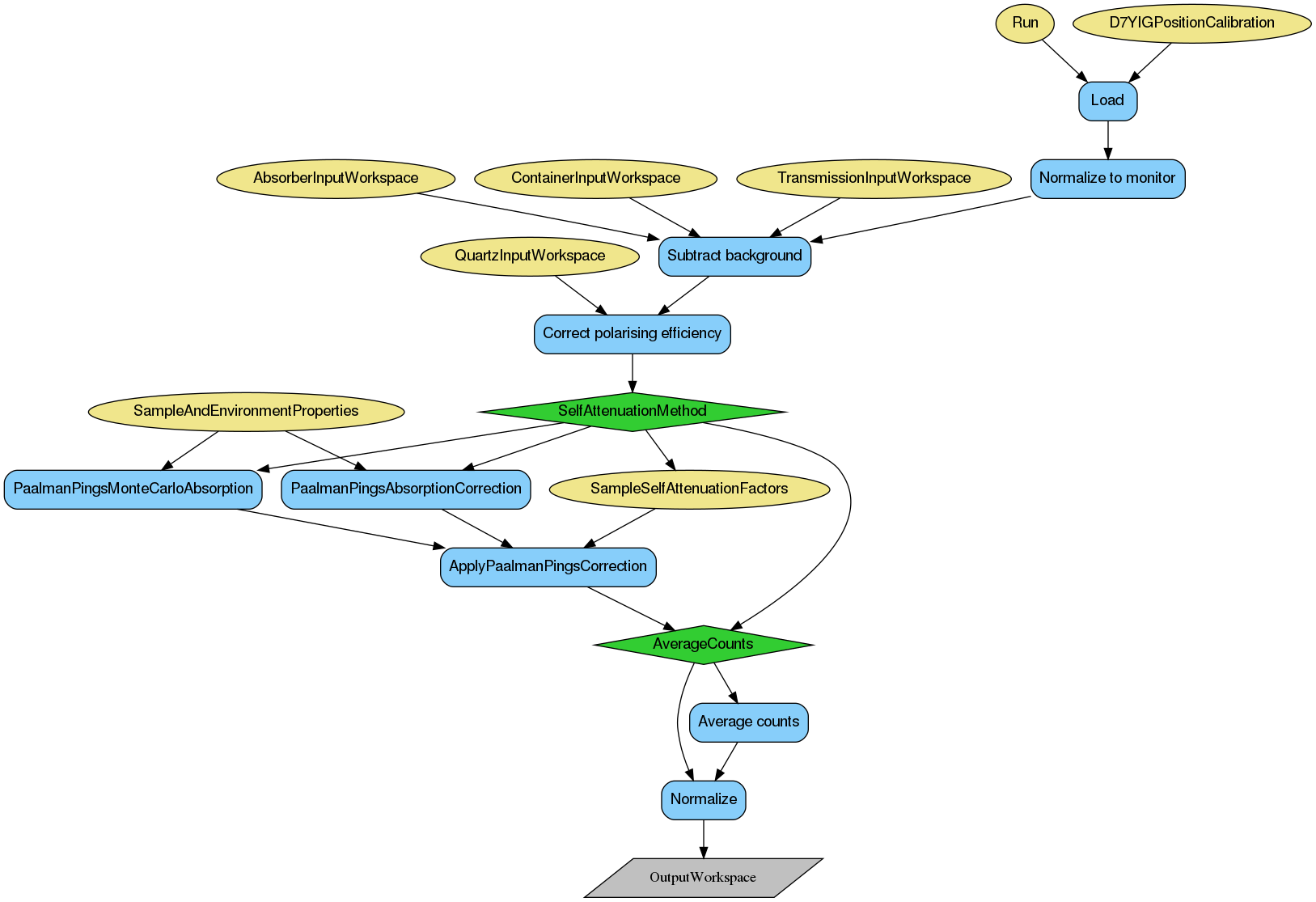
Vanadium provides a measure of the relative detector efficiencies and its count rate can be used for the calibration of sample data to absolute units. Multiple scattering and sample self-attenuation are issues here and the correction works best if the vanadium has, as close as possible, the same attenuation and shape as the sample.

The scattering from the vanadium is considered to be purely elastic scattering and the cross-section considered to be purely due to the nuclear spin-incoherent contribution. The reduced vanadium data can be used to normalise the results of the sample data reduction in D7AbsoluteCrossSections. The vanadium data can also be used as a consistency check for polarization and multiple scattering corrections.

If the sample has a large nuclear-spin-incoherent cross-section, this separated cross-section can be used as a self-correction for detector efficiency and even for shape effects from the sample. If the sample stoichiometry is well-known and an accurate estimate for the nuclear-spin-incoherent cross-section can be derived, this cross-section can be used to express the sample data in absolute units. In this case, the vanadium cross-section is unnecessary.

For the best results of using the reduced vanadium data as input for sample data normalisation, the OutputTreatment property of the PolDiffILLReduction algorithm needs to be set to Sum.

Reduction workflow ¶

The first two steps of the reduction of vanadium data are the same as for quartz, with normalisation to the monitor and background subtraction (provided the necessary inputs). The polarisation efficiency of the instrument can be corrected using the previously reduced quartz data. The correction is applied according to the following formula:

\[\begin{split}\begin{bmatrix} \dot{I_{B}}(+) \\ \dot{I_{B}}(-) \\ \end{bmatrix} = \frac{1}{2 f_{p} \phi} \begin{bmatrix} (1-\phi)(1-f_{p}) + f_{p}(1+\phi) & -(1-\phi) \\ -(1+\phi)(1-f_{p}) - f_{p}(1-\phi) & (1+\phi) \\ \end{bmatrix} \begin{bmatrix} \dot{I_{B}}(0) \\ \dot{I_{B}}(1) \\ \end{bmatrix},\end{split}\]

where \(\dot{I_{B}}(+)\) and \(\dot{I_{B}}(-)\) denote the spin-flip and the non-spin-flip scattering events, respectively, and \(\dot{I_{B}}(0)\) and \(\dot{I_{B}}(1)\) are the events with the flipper state on and off, respectively.

Self-attenuation correction ¶

There are three ways the self-attenuation of a sample can be taken into account in the implemented D7 reduction: Numerical, MonteCarlo, and User. In all three cases, the correction is applied to data with ApplyPaalmanPingsCorrection algorithm.

The User option depends on the self-attenuation parameters provided by the user through SampleSelfAttenuationFactors property of the PolDiffILLReduction algorithm. This option allows to study the self-attenuation of a sample that can have arbitrary shape separately from running the reduction algorithm, and in more detail if necessary.

On the contrary, The Numerical and MonteCarlo options calculate the self-attenuation parameters for both the sample and its container during the execution of the reduction algorithm. These two options depend on Mantid algorithms PaalmanPingsAbsorptionCorrection and PaalmanPingsMonteCarloAbsorption, respectively. These two algorithms require multiple parameters describing the sample and its environment, such as the geometry, density, and chemical composition to be defined. The communication of these parameters is done via SampleAndEnvironmentProperties property of the PolDiffILLReduction algorithm. All the necessary and accepted keys that need to be defined for the sample self-attenuation to be properly corrected are described below.

The SampleAndEnvironmentProperties property of the PolDiffILLReduction algorithm is a dictionary containing all of the information about the sample and its environment. This information is used in self-attenuation calculations and also can be reused in data normalisation in the D7AbsoluteCrossSections algorithm.

The complete list of keys can is summarised below:

Sample-only keys:

SampleMass
FormulaUnits
FormulaUnitMass
SampleChemicalFormula
SampleDensity
Height

The first three keys need to be always defined, so that the number of moles of the sample can be calculated, to ensure proper data normalisation. All of the density parameters are number density in formula units.

Container-only keys:

ContainerChemicalFormula
ContainerDensity

Optional beam-only keys, if not user-defined will be automatically defined to be larger than the sample dimensions:

BeamHeight
BeamWidth

Then, depending on the chosen sample geometry, additional parameters need to be defined:

For FlatPlate:
- SampleThickness
- SampleWidth
- SampleCenter
- SampleAngle
- ContainerFrontThickness
- ContainerBackThickness
For Cylinder:
- SampleRadius
- ContainerRadius
For Annulus:
- SampleInnerRadius
- SampleOuterRadius
- ContainerInnerRadius
- ContainerOuterRadius

Depending on the choice of the self-attenuation method, either ElementSize in case of numerical calculations or EventsPerPoint for Monte-Carlo method need to be defined.

Optional keys:

InitialEnergy - if not provided, the value will be calculated from the wavelength in the SampleLogs
NMoles - if not provided, the value will be calculated based on the SampleMass and FormulaUnitMass

Output ¶

The corrected counts in each each detector are normalised to the expected total cross-section for vanadium of \(0.404 \frac{\text{barn}}{\text{steradian} \cdot \text{atom}}\). The output of vanadium reduction is a WorkspaceGroup with one entry if the OutputTreatment is set to Sum, or the same number of entries as input data if Individual was selected.

In case it is desireable to separate cross-sections, for example for diagnostic purposes, it can be done using the reduced data described as above using D7AbsoluteCrossSections algorithm. More details on working with this algorithm are given in the sample normalisation section.

Workflow diagrams and working example ¶

Below is the relevant workflow diagram describing reduction steps of the vanadium reduction.

../_images/PolDiffILLReduction-v1_vanadium_wkflw.png

Note

To run these usage examples please first download the usage data, and add these to your path. In Mantid this is done using Manage User Directories.

Example - Vanadium reduction with annulus geometry

vanadium_dictionary = {'SampleMass':8.54,'FormulaUnits':1,'FormulaUnitMass':50.94,'SampleChemicalFormula':'V',
                       'Height':2.0,'SampleDensity':0.118,'SampleInnerRadius':2.0, 'SampleOuterRadius':2.49,
                       'BeamWidth':2.5,'BeamHeight':2.5,
                       'ContainerChemicalFormula':'Al','ContainerDensity':0.0027,'ContainerOuterRadius':2.52,
                       'ContainerInnerRadius':1.99, 'EventsPerPoint':1000}

calibration_file='D7_YIG_calibration.xml' # example calibration file

# Beam with cadmium absorber, used for transmission
PolDiffILLReduction(
    Run='396991',
    OutputWorkspace='cadmium_transmission_ws',
    ProcessAs='BeamWithCadmium'
)
# Beam measurement for transmisison
PolDiffILLReduction(
    Run='396983',
    OutputWorkspace='beam_ws',
    CadmiumTransmissionInputWorkspace='cadmium_transmission_ws_1',
    ProcessAs='EmptyBeam'
)

# Quartz transmission
PolDiffILLReduction(
    Run='396985',
    OutputWorkspace='quartz_transmission',
    CadmiumTransmissionInputWorkspace='cadmium_transmission_ws_1',
    BeamInputWorkspace='beam_ws_1',
    ProcessAs='Transmission'
)

# Empty container
PolDiffILLReduction(
    Run='396917',
    OutputWorkspace='empty_ws',
    ProcessAs='Empty'
)

# Absorber
PolDiffILLReduction(
    Run='396928',
    OutputWorkspace='cadmium_ws',
    ProcessAs='Cadmium'
)

# Polarisation correction
PolDiffILLReduction(
    Run='396939',
    OutputWorkspace='pol_corrections',
    CadmiumInputWorkspace='cadmium_ws',
    EmptyInputWorkspace='empty_ws',
    TransmissionInputWorkspace='quartz_transmission_1',
    OutputTreatment='Average',
    ProcessAs='Quartz'
)

# Vanadium transmission
PolDiffILLReduction(
    Run='396990',
    OutputWorkspace='vanadium_transmission',
    CadmiumTransmissionInputWorkspace='cadmium_transmission_ws_1',
    BeamInputWorkspace='beam_ws_1',
    ProcessAs='Transmission'
)
print('Vanadium transmission is {0:.3f}'.format(mtd['vanadium_transmission_1'].readY(0)[0]))

# Vanadium reduction
PolDiffILLReduction(
    Run='396993',
    OutputWorkspace='vanadium_ws',
    CadmiumInputWorkspace='cadmium_ws',
    EmptyInputWorkspace='empty_ws',
    TransmissionInputWorkspace='vanadium_transmission_1',
    QuartzInputWorkspace='pol_corrections',
    OutputTreatment='Sum',
    SelfAttenuationMethod='MonteCarlo',
    SampleGeometry='Annulus',
    SampleAndEnvironmentProperties=vanadium_dictionary,
    InstrumentCalibration=calibration_file,
    ProcessAs='Vanadium'
)
print("The vanadium reduction output contains {} entry with {} spectra and {} bin.".format(mtd['vanadium_ws'].getNumberOfEntries(),
          mtd['vanadium_ws'][0].getNumberHistograms(), mtd['vanadium_ws'][0].blocksize()))

Output:

Vanadium transmission is 0.886
The vanadium reduction output contains 1 entry with 132 spectra and 1 bin.

Sample data reduction ¶

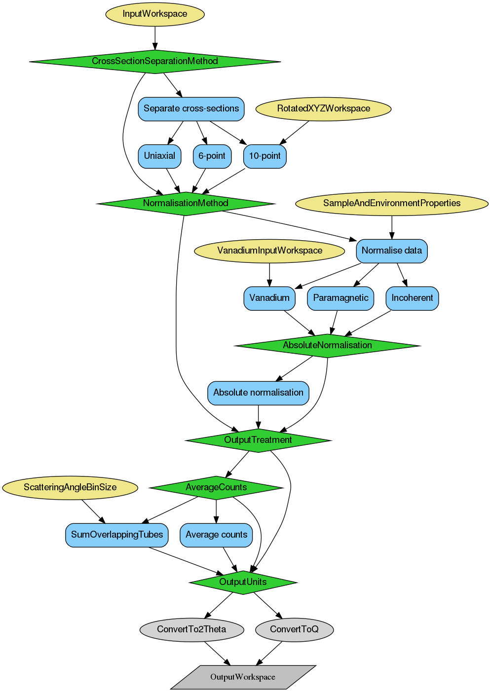
The sample data reduction follows the same steps of monitor normalisation, background subtraction, polarisation correction, and self-attenuation correction as vanadium data reduction. Should the self-attenuation correction be taken into account, the relevant sample and environment parameters need to be defined in a dictionary that is provided to SampleAndEnvironmentProperty with keys described in the vanadium reduction section.

The output of the is a WorkspaceGroup with the number of entries equal to number of measured polarisations times number of steps in a \(2\theta\) scan. This output can be provided to D7AbsoluteCrossSections for cross-section separation, e.g. for diagnostic purposes, or for the final normalisation.

Cross-section separation ¶

The D7AbsoluteCrossSections algorithm allows for either cross-section separation or sample data normalisation. It is possible to use only one of the possibilities, for example, to separate cross-sections of the reduced vanadium data without the normalisation subroutines to be invoked. This is especially useful for diagnostic purposes.

The cross-section separation is done according to formulae presented in Ref. [3] [4] [5]. More details on the exact calculations is given in documentation of the D7AbsoluteCrossSections algorithm. It is possible to perform uniaxial, 6-point (or XYZ), and 10-point measurement separation of magnetic, nuclear coherent, and nuclear-spin-incoherent components of the total measured scattering cross-section. The specifics of the 10-point measurement as a set of two separate 6-point measurements are taken into account. In that case, the second set of 6-point data needs to be provided to RotatedXYZWorkspace property of the D7AbsoluteCrossSections algorithm, and the ‘10-p’ needs to be chosen as the CrossSectionSeparationMethod.

Sample data normalisation ¶

The output from sample data reduction still needs to be normalised to the relevant standard to set the units to absolute scale. The normalisation is handled by D7AbsoluteCrossSections algorithm, and there are three options available to normalise the sample data:

Vanadium normalisation

Uses output from the vanadium data reduction. The units chosen for both the sample and vanadium data during reduction should agree.
Paramagnetic normalisation

This normalisation approach uses the output from the cross-section separation to set the sample output to absolute units. An additional parameter needs to be defined in the sample properties dictionary, named SampleSpin, to define the spin of the sample.
Spin-incoherent normalisation

This normalisation approach also uses the output from the cross-section separation. If the goal is to set the output data to absolute scale, an additional parameter needs to be defined in the sample properties dictionary, named IncoherentCrossSection, to provide the total nuclear-spin-incoherent cross-section of the sample.

In all cases, a relative normalisation to the detector with highest number of counts is always performed.

Output ¶

The output of the reduction and normalisation is a WorkspaceGroup with the number of entries consistent with the input if the OutputTreatment property was selected to be Individual, or the number of entries will be consistent with either the number of polarisation orientations present in the data (e.g. six for a XYZ method) or the number of separated cross-section. Each entry of the output group is a workspace with X-axis unit being either momentum exchange \(Q\) or the scattering angle \(2\theta\).

Workflow diagrams and working example ¶

Below is the relevant workflow diagram describing reduction steps of the sample reduction and normalisation.

Sample reduction ¶

../_images/PolDiffILLReduction-v1_sample_wkflw.png

Sample normalisation ¶

../_images/D7AbsoluteCrossSections-v1_wkflw.png

Note

To run these usage examples please first download the usage data, and add these to your path. In Mantid this is done using Manage User Directories.

Example - Complete sample reduction with normalisation

vanadium_dictionary = {'SampleMass':8.54,'FormulaUnits':1,'FormulaUnitMass':50.94}

sample_dictionary = {'SampleMass':2.932,'SampleDensity':2.0,'FormulaUnits':1,'FormulaUnitMass':182.56,
                     'SampleChemicalFormula':'Mn0.5-Fe0.5-P-S3','Height':2.0,'SampleDensity':0.118,
                     'SampleInnerRadius':2.0, 'SampleOuterRadius':2.49,'BeamWidth':2.5,'BeamHeight':2.5,
                     'ContainerChemicalFormula':'Al','ContainerDensity':0.027,'ContainerOuterRadius':2.52,
                     'ContainerInnerRadius':1.99, 'ElementSize':0.5}

calibration_file = 'D7_YIG_calibration.xml'

# Beam with cadmium absorber, used for transmission
PolDiffILLReduction(
    Run='396991',
    OutputWorkspace='cadmium_transmission_ws',
    ProcessAs='BeamWithCadmium'
)
# Beam measurement for transmisison
PolDiffILLReduction(
    Run='396983',
    OutputWorkspace='beam_ws',
    CadmiumTransmissionInputWorkspace='cadmium_transmission_ws_1',
    ProcessAs='EmptyBeam'
)

# Quartz transmission
PolDiffILLReduction(
    Run='396985, 396986',
    OutputWorkspace='quartz_transmission',
    CadmiumTransmissionInputWorkspace='cadmium_transmission_ws_1',
    BeamInputWorkspace='beam_ws_1',
    ProcessAs='Transmission'
)

# Empty container
PolDiffILLReduction(
    Run='396917, 396918',
    OutputWorkspace='empty_ws',
    ProcessAs='Empty'
)

# Cadmium absorber
PolDiffILLReduction(
    Run='396928, 396929',
    OutputWorkspace='cadmium_ws',
    ProcessAs='Cadmium'
)

# Polarisation correction
PolDiffILLReduction(
    Run='396939, 396940',
    OutputWorkspace='pol_corrections',
    CadmiumInputWorkspace='cadmium_ws',
    EmptyInputWorkspace='empty_ws',
    TransmissionInputWorkspace='quartz_transmission_1',
    OutputTreatment='Average',
    ProcessAs='Quartz'
)

# Vanadium transmission
PolDiffILLReduction(
    Run='396990',
    OutputWorkspace='vanadium_transmission',
    CadmiumTransmissionInputWorkspace='cadmium_transmission_ws_1',
    BeamInputWorkspace='beam_ws_1',
    ProcessAs='Transmission'
)

# Vanadium reduction
PolDiffILLReduction(
    Run='396993, 396994',
    OutputWorkspace='vanadium_ws',
    CadmiumInputWorkspace='cadmium_ws',
    EmptyInputWorkspace='empty_ws',
    TransmissionInputWorkspace='vanadium_transmission_1',
    QuartzInputWorkspace='pol_corrections',
    OutputTreatment='Sum',
    SampleGeometry='None',
    SampleAndEnvironmentProperties=vanadium_dictionary,
    AbsoluteNormalisation=True,
    InstrumentCalibration=calibration_file,
    ProcessAs='Vanadium'
)
# Sample transmission
PolDiffILLReduction(
   Run='396986, 396987',
   OutputWorkspace='sample_transmission',
   CadmiumTransmissionInputWorkspace='cadmium_transmission_ws_1',
   BeamInputWorkspace='beam_ws_1',
   ProcessAs='Transmission'
)
print('Sample transmission is {0:.3f}'.format(mtd['sample_transmission_1'].readY(0)[0]))

# Sample reduction
PolDiffILLReduction(
    Run='397004, 397005',
    OutputWorkspace='sample_ws',
    CadmiumInputWorkspace='cadmium_ws',
    EmptyInputWorkspace='empty_ws',
    TransmissionInputWorkspace='sample_transmission_1',
    QuartzInputWorkspace='pol_corrections',
    OutputTreatment='Individual',
    InstrumentCalibration=calibration_file,
    SelfAttenuationMethod='Numerical',
    SampleGeometry='Annulus',
    SampleAndEnvironmentProperties=sample_dictionary,
    ProcessAs='Sample'
)
print("The reduced sample data contains {} entries with {} spectra and {} bins.".format(mtd['sample_ws'].getNumberOfEntries(),
          mtd['sample_ws'][0].getNumberHistograms(), mtd['sample_ws'][0].blocksize()))

# Normalise sample data
D7AbsoluteCrossSections(
    InputWorkspace='sample_ws',
    OutputWorkspace='sample_norm',
    CrossSectionSeparationMethod='None',
    NormalisationMethod='Vanadium',
    VanadiumInputWorkspace='vanadium_ws',
    OutputTreatment='Merge',
    OutputUnits='TwoTheta',
    ScatteringAngleBinSize=1.0, # degrees
    SampleAndEnvironmentProperties=sample_dictionary,
    AbsoluteUnitsNormalisation=False
)

print("The normalised sample data contains {} entries with {} spectrum and {} bins.".format(mtd['sample_norm'].getNumberOfEntries(),
          mtd['sample_norm'][0].getNumberHistograms(), mtd['sample_norm'][0].blocksize()))

Output:

Sample transmission is 0.962
The reduced sample data contains 12 entries with 132 spectra and 1 bins.
The normalised sample data contains 6 entries with 1 spectrum and 134 bins.

References ¶

[1]	T. Fennell, L. Mangin-Thro, H.Mutka, G.J. Nilsen, A.R. Wildes. Wavevector and energy resolution of the polarized diffuse scattering spectrometer D7, Nuclear Instruments and Methods in Physics Research A 857 (2017) 24–30 doi: 10.1016/j.nima.2017.03.024

[2]	A. Nakatsuka, A. Yoshiasa, and S. Takeno. Site preference of cations and structural variation in Y3Fe5O12 solid solutions with garnet structure, Acta Crystallographica Section B 51 (1995) 737–745 doi: 10.1107/S0108768194014813

[3]	Scharpf, O. and Capellmann, H. The XYZ‐Difference Method with Polarized Neutrons and the Separation of Coherent, Spin Incoherent, and Magnetic Scattering Cross Sections in a Multidetector Physica Status Solidi (A) 135 (1993) 359-379 doi: 10.1002/pssa.2211350204

[4]

Stewart, J. R. and Deen, P. P. and Andersen, K. H. and Schober, H. and Barthelemy, J.-F. and Hillier, J. M. and Murani, A. P. and Hayes, T. and Lindenau, B. Disordered materials studied using neutron polarization analysis on the multi-detector spectrometer, D7 Journal of Applied Crystallography 42 (2009) 69-84 doi: 10.1107/S0021889808039162

[5]	G. Ehlers, J. R. Stewart, A. R. Wildes, P. P. Deen, and K. H. Andersen Generalization of the classical xyz-polarization analysis technique to out-of-plane and inelastic scattering Review of Scientific Instruments 84 (2013), 093901 doi: 10.1063/1.4819739

Category: Techniques