\(\renewcommand\AA{\unicode{x212B}}\)
AbsorptionCorrection dialog.
Table of Contents
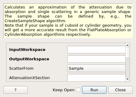
Calculates an approximation of the attenuation due to absorption and single scattering in a generic sample shape. The sample shape can be defined by, e.g., the CreateSampleShape algorithm. Note that if your sample is of cuboid or cylinder geometry, you will get a more accurate result from the FlatPlateAbsorption or CylinderAbsorption algorithms respectively.
| Name | Direction | Type | Default | Description |
|---|---|---|---|---|
| InputWorkspace | Input | MatrixWorkspace | Mandatory | The X values for the input workspace must be in units of wavelength |
| OutputWorkspace | Output | MatrixWorkspace | Mandatory | Output workspace name |
| ScatterFrom | Input | string | Sample | The component to calculate the absorption for (default: Sample). Allowed values: [‘Sample’, ‘Container’, ‘Environment’] |
| AttenuationXSection | Input | number | Optional | The ABSORPTION cross-section, at 1.8 Angstroms, for the sample material in barns. Column 8 of a table generated from http://www.ncnr.nist.gov/resources/n-lengths/. |
| ScatteringXSection | Input | number | Optional | The (coherent + incoherent) scattering cross-section for the sample material in barns. Column 7 of a table generated from http://www.ncnr.nist.gov/resources/n-lengths/. |
| SampleNumberDensity | Input | number | Optional | The number density of the sample in number of atoms per cubic angstrom if not set with SetSampleMaterial |
| NumberOfWavelengthPoints | Input | number | Optional | The number of wavelength points for which the numerical integral is calculated (default: all points) |
| ExpMethod | Input | string | Normal | Select the method to use to calculate exponentials, normal or a fast approximation (default: Normal). Allowed values: [‘Normal’, ‘FastApprox’] |
| EMode | Input | string | Elastic | The energy mode (default: elastic). Allowed values: [‘Elastic’, ‘Direct’, ‘Indirect’] |
| EFixed | Input | number | 0 | The value of the initial or final energy, as appropriate, in meV. Will be taken from the instrument definition file, if available. |
| ElementSize | Input | number | 1 | The size of one side of an integration element cube in mm |
This algorithm uses a numerical integration method to calculate attenuation factors resulting from absorption and single scattering in a sample with the material properties given. Factors are calculated for each spectrum (i.e. detector position) and wavelength point, as defined by the input workspace. The sample is first bounded by a cuboid, which is divided up into small cubes. The cubes whose centres lie within the sample make up the set of integration elements (so you have a kind of ‘Lego’ model of the sample) and path lengths through the sample are calculated for the centre-point of each element, and a numerical integration is carried out using these path lengths over the volume elements.
The output workspace will contain the attenuation factors. To apply the correction you must divide your data set by the resulting factors.
Note that the duration of this algorithm is strongly dependent on the element size chosen, and that too small an element size can cause the algorithm to fail because of insufficient memory.
Note that The number density of the sample is in \(\mathrm{\AA}^{-3}\)
This flow chart is given as a way of selecting the most appropriate of
the absorption correction algorithms. It also shows the algorithms that
must be run first in each case. Note that this does not cover the
following absorption correction algorithms:
MonteCarloAbsorption v1 (correction factors for
a generic sample using a Monte Carlo instead of a numerical integration
method),
CarpenterSampleCorrection v1
& AnvredCorrection v1 (corrections in a spherical
sample, using a method imported from ISAW). Also, HRPD users can use the
HRPDSlabCanAbsorption v1 to add rudimentary
calculations of the effects of the sample holder. 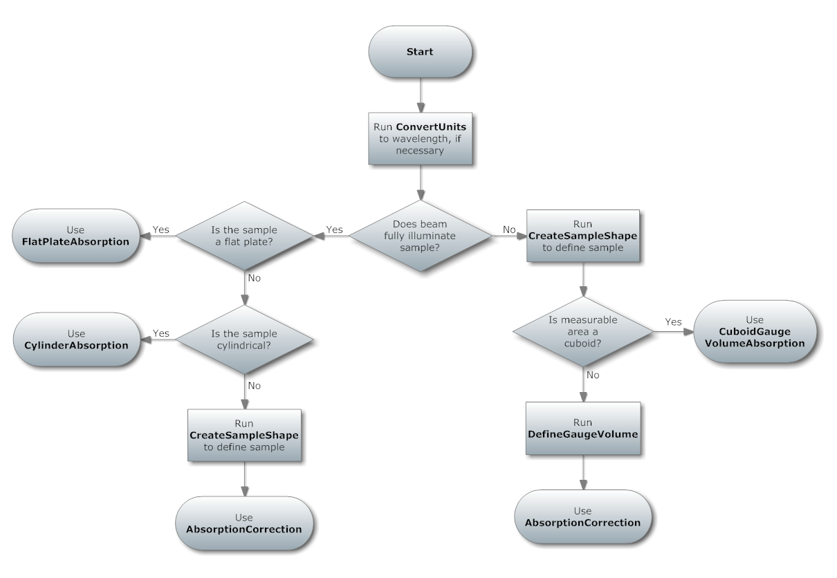
This algorithm assumes that the (parallel) beam illuminates the entire sample unless a ‘gauge volume’ has been defined using the DefineGaugeVolume v1 algorithm (or by otherwise adding a valid XML string defining a shape to a Run property called “GaugeVolume”). In this latter case only scattering within this volume (and the sample) is integrated, because this is all the detector can ‘see’. The full sample is still used for the neutron paths. (N.B. If your gauge volume is of axis-aligned cuboid shape and fully enclosed by the sample then you will get a more accurate result from the CuboidGaugeVolumeAbsorption v1 algorithm.)
The input workspace must have units of wavelength. The instrument associated with the workspace must be fully defined because detector, source & sample position are needed.
Example: A simple spherical sample
#setup the sample shape
sphere = '''<sphere id="sample-sphere">
<centre x="0" y="0" z="0"/>
<radius val="0.1" />
</sphere>'''

ws = CreateSampleWorkspace("Histogram",NumBanks=1,BankPixelWidth=1)
ws = ConvertUnits(ws,"Wavelength")
ws = Rebin(ws,Params=[1])
CreateSampleShape(ws,sphere)
SetSampleMaterial(ws,ChemicalFormula="V")

#restrict the number of wavelength points to speed up the example
wsOut = AbsorptionCorrection(ws, NumberOfWavelengthPoints=5, ElementSize=3)
wsCorrected = ws / wsOut

print("The created workspace has one entry for each spectra: {}".format(wsOut.getNumberHistograms()))
print("Original y values:  {}".format(ws.readY(0)))
print("Corrected y values:  {}".format(wsCorrected.readY(0)))
Output:
The created workspace has one entry for each spectra: 1
Original y values:  [  5.68751434   5.68751434  15.68751434   5.68751434   5.68751434
   1.56242829]
Corrected y values:  [   818.39955533   2377.16206099  14230.46290595   9497.08390031
  15787.69382575   5780.15301643]
Categories: AlgorithmIndex | CorrectionFunctions\AbsorptionCorrections