\(\renewcommand\AA{\unicode{x212B}}\)

DoublePulseFit v1¶

DoublePulseFit dialog.

Table of Contents

Summary
- See Also
Properties
Description
Usage
Source

Summary ¶

A function to fit muon data from a double pulse source. Wraps Fit.

Properties ¶

Name	Direction	Type	Default	Description
Function	InOut	Function	Mandatory	Parameters defining the fitting function and its initial values
InputWorkspace	Input	Workspace	Mandatory	Name of the input Workspace
IgnoreInvalidData	Input	boolean	False	Flag to ignore infinities, NaNs and data with zero errors.
DomainType	Input	string	Simple	The type of function domain to use: Simple, Sequential, or Parallel. Allowed values: [‘Simple’, ‘Sequential’, ‘Parallel’]
EvaluationType	Input	string	CentrePoint	The way the function is evaluated on histogram data sets. If value is “CentrePoint” then function is evaluated at centre of each bin. If it is “Histogram” then function is integrated within the bin and the integrals returned. Allowed values: [‘CentrePoint’, ‘Histogram’]
PeakRadius	Input	number	0	A value of the peak radius the peak functions should use. A peak radius defines an interval on the x axis around the centre of the peak where its values are calculated. Values outside the interval are not calculated and assumed zeros.Numerically the radius is a whole number of peak widths (FWHM) that fit into the interval on each side from the centre. The default value of 0 means the whole x axis.
Ties	Input	string		Math expressions defining ties between parameters of the fitting function.
Constraints	Input	string		List of constraints
MaxIterations	Input	number	500	Stop after this number of iterations if a good fit is not found
OutputStatus	Output	string		Whether the fit was successful
OutputChi2overDoF	Output	number		Returns the goodness of the fit
Minimizer	Input	string	Levenberg-Marquardt	Minimizer to use for fitting. Allowed values: [‘BFGS’, ‘Conjugate gradient (Fletcher-Reeves imp.)’, ‘Conjugate gradient (Polak-Ribiere imp.)’, ‘Damped GaussNewton’, ‘FABADA’, ‘Levenberg-Marquardt’, ‘Levenberg-MarquardtMD’, ‘Simplex’, ‘SteepestDescent’, ‘Trust Region’]
CostFunction	InOut	string	Least squares	The cost function to be used for the fit, default is Least squares. Allowed values: [‘Least squares’, ‘Poisson’, ‘Rwp’, ‘Unweighted least squares’]
CreateOutput	Input	boolean	False	Set to true to create output workspaces with the results of the fit(default is false).
Output	Input	string		A base name for the output workspaces (if not given default names will be created). The default is to use the name of the original data workspace as prefix followed by suffixes _Workspace, _Parameters, etc.
CalcErrors	Input	boolean	False	Set to true to calcuate errors when output isn’t created (default is false).
OutputCompositeMembers	Input	boolean	False	If true and CreateOutput is true then the value of each member of a Composite Function is also output.
ConvolveMembers	Input	boolean	False	If true and OutputCompositeMembers is true members of any Convolution are output convolved with corresponding resolution
OutputParametersOnly	Input	boolean	False	Set to true to output only the parameters and not workspace(s) with the calculated values (default is false, ignored if CreateOutput is false and Output is an empty string).
PulseOffset	Input	number	0	The time offset between the two pulses
FirstPulseWeight	Input	number	0.5	Weighting of first pulse.
SecondPulseWeight	Input	number	0.5	Weighting of second pulse.

Description ¶

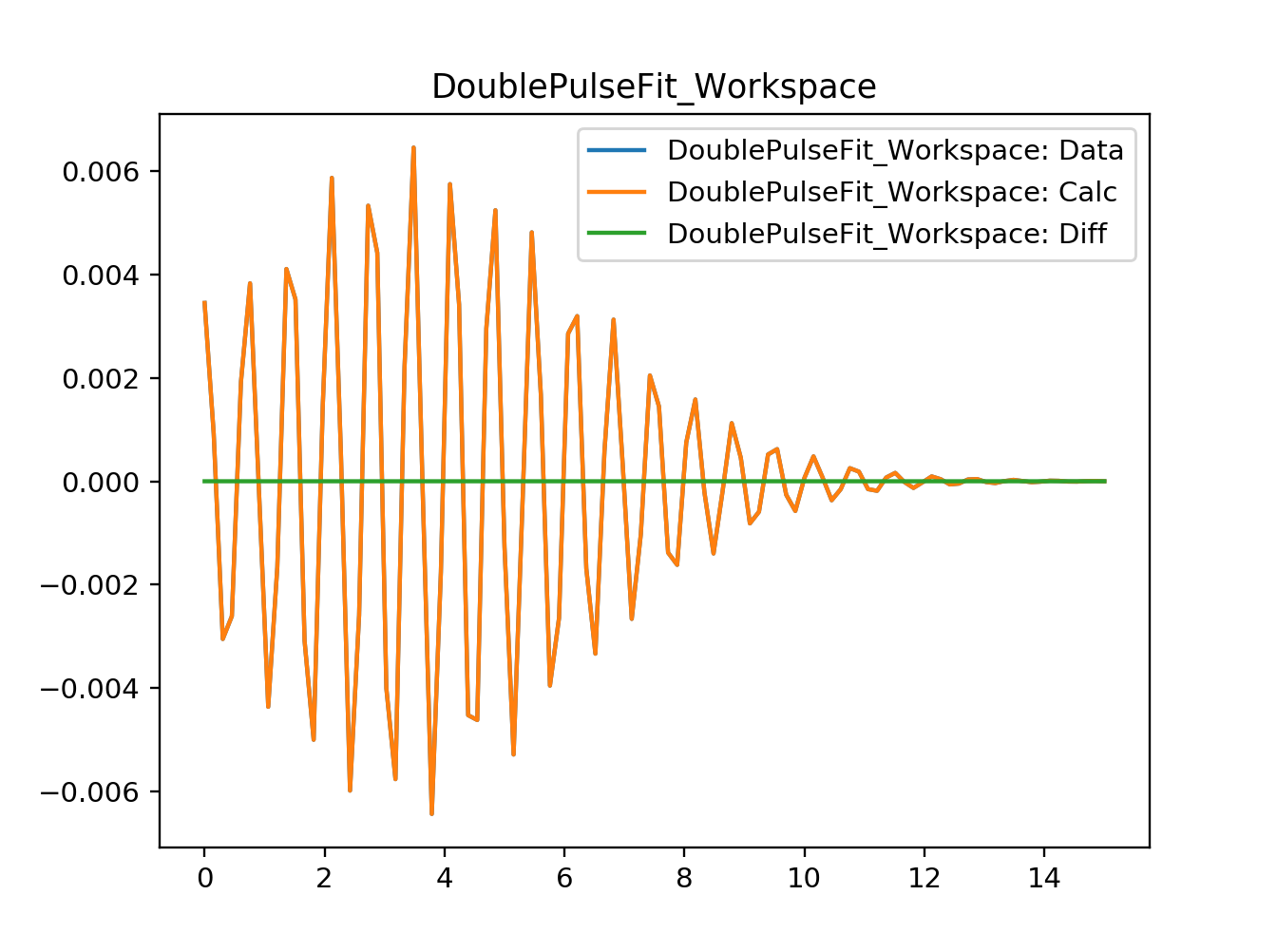
This algorithm is is designed to analyse double pulse Muon data. It fits two copies of the input function seperated by a time offset. The function fitted is of the form

\[f(t) = N_1 f(t + t_s/2)_{input} + N_2 f(t - t_s/2)_{input},\]

where \(N_1\) is the FirstPulseWeight, \(N_2\) is the SecondPulseWeight and \(t_s\) is the PulseOffset. The corresponding parameters of the two input functions are tied to have the same value. In practise this is achieved by taking a convolution of two delta functions with the input function;

\[f(t) = f(t)_{input} * (N_1\delta(-t_s/2) + N_2\delta(t_s/2)).\]

With the exception of the three new parameters PulseOffset, FirstPulseWeight and SecondPulseWeight the interface for DoublePulseFit is identical to that of Fit and the two can be used interchangeably. The function output by this algorithm corrospond to the inner function only whilst the output fit curves corrospond to the full function.

Usage ¶

import numpy as np
from mantid.simpleapi import DoublePulseFit, CreateWorkspace, GausOsc, Fit
from mantid.api import FunctionFactory, AnalysisDataService

# Create a workspace with two offset oscillations
delta = 0.33
x = np.linspace(0.,15.,100)
x_offset = np.linspace(delta/2, 15. + delta/2, 100)
x_offset_neg = np.linspace(-delta/2, 15. - delta/2, 100)

testFunction = GausOsc(Frequency = 1.5, A=0.22)
y1 = testFunction(x_offset_neg)
y2 = testFunction(x_offset)
y = y1/2+y2/2
ws = CreateWorkspace(x,y)

# Create functions to fit
convolution =  FunctionFactory.createCompositeFunction('Convolution')
innerFunction = FunctionFactory.createInitialized('name=GausOsc,A=0.2,Sigma=0.2,Frequency=1,Phi=0')
deltaFunctions = FunctionFactory.createInitialized('(name=DeltaFunction,Height=0.5,Centre={},ties=(Height=0.5,Centre={});name=DeltaFunction,Height=0.5,Centre={},ties=(Height=0.5,Centre={}))'.format(-delta/2, -delta/2, delta/2, delta/2))
convolution.setAttributeValue('FixResolution', False)
convolution.add(innerFunction)
convolution.add(deltaFunctions)
innerFunctionSingle = FunctionFactory.createInitialized('name=GausOsc,A=0.2,Sigma=0.2,Frequency=1,Phi=0')

DoublePulseFit(Function=innerFunctionSingle, InputWorkspace=ws,  PulseOffset = delta, StartX=0.0, EndX=15.0, Output='DoublePulseFit')
Fit(Function=convolution, InputWorkspace=ws, CreateOutput = True, StartX=0.0, EndX=15.0, Output='Fit')

double_parameter_workspace = AnalysisDataService.retrieve('DoublePulseFit_Parameters')
double_col_values = double_parameter_workspace.column(1)

single_parameter_workspace = AnalysisDataService.retrieve('Fit_Parameters')
col_values = single_parameter_workspace.column(1)

print('Fitted value of A from DoublePulseFit is {:.2g}'.format(double_col_values[0]))
print('Fitted value of Frequency from DoublePulseFit is {:.2g}'.format(double_col_values[2]))
print('Fitted value of A from Fit is {:.2g}'.format(col_values[0]))
print('Fitted value of Frequency from Fit is {:.2g}'.format(col_values[2]))

Output:

Fitted value of A from DoublePulseFit is 0.22
Fitted value of Frequency from DoublePulseFit is 1.5
Fitted value of A from Fit is 0.22
Fitted value of Frequency from Fit is 1.5