\(\renewcommand\AA{\unicode{x212B}}\)
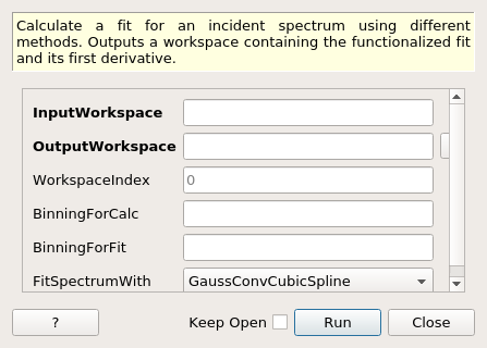
FitIncidentSpectrum dialog.
Table of Contents
Calculate a fit for an incident spectrum using different methods. Outputs a workspace containing the functionalized fit and its first derivative.
| Name | Direction | Type | Default | Description |
|---|---|---|---|---|
| InputWorkspace | Input | MatrixWorkspace | Mandatory | Incident spectrum to be fit. |
| OutputWorkspace | Output | MatrixWorkspace | Mandatory | Output workspace containing the fit and it’s first derivative. |
| WorkspaceIndex | Input | number | 0 | Workspace index of the spectra to be fitted (Defaults to the first index.) |
| BinningForCalc | Input | dbl list | Bin range for calculation given as an array of floats in the same format as Rebin: [Start],[Increment],[End]. If empty use default binning. The calculated spectrum will use this binning | |
| BinningForFit | Input | dbl list | Bin range for fitting given as an array of floats in the same format as Rebin: [Start],[Increment],[End]. If empty use BinningForCalc. The incident spectrum will be rebined to this range before being fit. | |
| FitSpectrumWith | Input | string | GaussConvCubicSpline | The method for fitting the incident spectrum. Allowed values: [‘GaussConvCubicSpline’, ‘CubicSpline’, ‘CubicSplineViaMantid’] |
This algorithm fits and functionalizes an incident spectrum and finds its first derivative. FitIncidentSpectrum is able to fit an incident spectrum using:
Example: fit an incident spectrum using GaussConvCubicSpline [1]
import numpy as np
import matplotlib.pyplot as plt
from mantid.simpleapi import \
    AnalysisDataService, \
    CalculateEfficiencyCorrection, \
    ConvertToPointData, \
    CreateWorkspace, \
    Divide, \
    FitIncidentSpectrum, \
    Rebin

# Create the workspace to hold the already corrected incident spectrum
incident_wksp_name = 'incident_spectrum_wksp'
binning_incident = "%s,%s,%s" % (0.2, 0.01, 4.0)
binning_for_calc = "%s,%s,%s" % (0.2, 0.2, 4.0)
binning_for_fit = "%s,%s,%s" % (0.2, 0.01, 4.0)
incident_wksp = CreateWorkspace(
    OutputWorkspace=incident_wksp_name,
    NSpec=1,
    DataX=[0],
    DataY=[0],
    UnitX='Wavelength',
    VerticalAxisUnit='Text',
    VerticalAxisValues='IncidentSpectrum')
incident_wksp = Rebin(InputWorkspace=incident_wksp, Params=binning_incident)
incident_wksp = ConvertToPointData(InputWorkspace=incident_wksp)


# Spectrum function given in Milder et al. Eq (5)
def incidentSpectrum(wavelengths, phiMax, phiEpi, alpha, lambda1, lambda2,
                     lamdaT):
    deltaTerm = 1. / (1. + np.exp((wavelengths - lambda1) / lambda2))
    term1 = phiMax * (
        lambdaT**4. / wavelengths**5.) * np.exp(-(lambdaT / wavelengths)**2.)
    term2 = phiEpi * deltaTerm / (wavelengths**(1 + 2 * alpha))
    return term1 + term2


# Variables for polyethlyene moderator at 300K
phiMax = 6324
phiEpi = 786
alpha = 0.099
lambda1 = 0.67143
lambda2 = 0.06075
lambdaT = 1.58

# Add the incident spectrum to the workspace
corrected_spectrum = incidentSpectrum(
    incident_wksp.readX(0), phiMax, phiEpi, alpha, lambda1, lambda2, lambdaT)
incident_wksp.setY(0, corrected_spectrum)

# Calculate the efficiency correction for Alpha=0.693
# and back calculate measured spectrum
eff_wksp = CalculateEfficiencyCorrection(
    InputWorkspace=incident_wksp, Alpha=0.693)
measured_wksp = Divide(LHSWorkspace=incident_wksp, RHSWorkspace=eff_wksp)

# Fit incident spectrum
prefix = "incident_spectrum_fit_with_"

fit_gauss_conv_spline = prefix + "_gauss_conv_spline"
FitIncidentSpectrum(
    InputWorkspace=incident_wksp,
    OutputWorkspace=fit_gauss_conv_spline,
    BinningForCalc=binning_for_calc,
    BinningForFit=binning_for_fit,
    FitSpectrumWith="GaussConvCubicSpline")

# Retrieve workspaces
wksp_fit_gauss_conv_spline = AnalysisDataService.retrieve(
    fit_gauss_conv_spline)

print(wksp_fit_gauss_conv_spline.readY(0))
Output:
[ 66366.97907003  35201.51411451  38022.36591024  61639.70236933
  62200.67498428  48463.5664824   34224.33749995  23402.41931673
  15942.7518712   10958.256381     7639.47147804   5413.27854911
   3900.21888036   2855.91654087   2123.40417572   1601.53146103
   1224.09479598    947.1952884 ]
| [1] |
|
Categories: AlgorithmIndex | Diffraction\Fitting
Python: FitIncidentSpectrum.py