\(\renewcommand\AA{\unicode{x212B}}\)
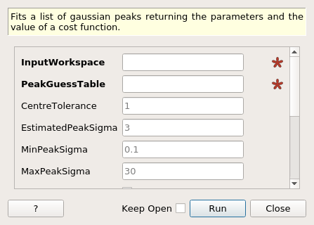
FitGaussianPeaks dialog.
Table of Contents
| Name | Direction | Type | Default | Description |
|---|---|---|---|---|
| InputWorkspace | Input | Workspace | Mandatory | Workspace with peaks to be identified |
| PeakGuessTable | Input | TableWorkspace | Mandatory | Table containing the guess for the peak position |
| CentreTolerance | Input | number | 1 | Tolerance value used in looking for peak centre |
| EstimatedPeakSigma | Input | number | 3 | Estimate of the peak half width |
| MinPeakSigma | Input | number | 0.1 | Minimum value for the standard deviation of a peak |
| MaxPeakSigma | Input | number | 30 | Maximum value for the standard deviation of a peak |
| EstimateFitWindow | Input | boolean | True | If checked, algorithm attempts to calculate number of data points to use from EstimatePeakSigma, if unchecked algorithm will use FitWindowSize argument |
| FitWindowSize | Input | number | 5 | Number of data point used to fit peaks, minimum allowed value is 5, value must be an odd number |
| GeneralFitTolerance | Input | number | 0.1 | Tolerance for the constraint in the general fit |
| RefitTolerance | Input | number | 0.001 | Tolerance for the constraint in the refitting |
| PeakProperties | Output | TableWorkspace | peak_table | Table containing the properties of the peaks |
| RefitPeakProperties | Output | TableWorkspace | refit_peak_table | Table containing the properties of the peaks that had to be fitted twice as the firsttime the error was unreasonably large |
| FitCost | Output | TableWorkspace | fit_cost | Table containing the value of both chi2 and poisson cost functions for the fit |
The algorithm takes:
It then performs the following steps:
The result of the fit is compared with the data using the equation: \({1 \over N} \sum_{i=1}^{N} {(m_i - d_i) \over \sigma_i}^2\)
Where \(m_i\) is the i-th data point of the result of the fit, \(d_i\) is the i-th data point of the data to be fitted and \(\sigma_i\) is the error on the i-th data point.
The result of the fit and input data are filtered to remove zeros in the fitted data. They are then compared using the equation: \(\sum_{i=1}^{N} (-m_i + d_i \ln(m_i))\)
Where \(m_i\) is the i-th data point of the result of the fit and \(d_i\) is the i-th data point of the data to be fitted. This is the natural logarithm of the cost, calculated as: \(\prod_{i=1}^{N} \exp(-m_i + d_i \ln(m_i))\)
Example - Finding two simple gaussian peaks.
# Function for a gaussian peak
def gaussian(xvals, centre, height, sigma):
    exp_val = (xvals - centre) / (np.sqrt(2) * sigma)

    return height * np.exp(-exp_val * exp_val)


# Creating two peaks
x_values = np.linspace(0, 100, 1001)
centre = [25, 75]
height = [35, 20]
width = [10, 5]
y_values = gaussian(x_values, centre[0], height[0], width[0])
y_values += gaussian(x_values, centre[1], height[1], width[1])
background = 10 * np.ones(len(x_values))

# Generating a table with a guess of the position of the centre of the peaks
peak_table = CreateEmptyTableWorkspace()
peak_table.addColumn(type='float', name='Approximated Centre')
peak_table.addRow([centre[0]+2])
peak_table.addRow([centre[1]-3])

# Generating a workspace with the data and a flat background
data_ws = CreateWorkspace(DataX=np.concatenate((x_values, x_values)),
                          DataY=np.concatenate((y_values, background)),
                          DataE=np.sqrt(np.concatenate((y_values, background))),
                          NSpec=2)

# Fitting the data
parameters, refitted_parameters, cost = FitGaussianPeaks(
    InputWorkspace=data_ws,
    PeakGuessTable=peak_table,
    CentreTolerance=3.0,
    EstimatedPeakSigma=5,
    MinPeakSigma=0.0,
    MaxPeakSigma=30.0,
    GeneralFitTolerance=0.1,
    RefitTolerance=0.001
)

peak1 = parameters.row(0)
peak2 = parameters.row(1)
print('Peak 1: centre={:.2f}+/-{:.2f}, height={:.2f}+/-{:.2f}, sigma={:.2f}+/-{:.1f}'
      .format(peak1['centre'], peak1['error centre'],
              peak1['height'], peak1['error height'],
              peak1['sigma'], peak1['error sigma']))
print('Peak 2: centre={:.2f}+/-{:.2f}, height={:.2f}+/-{:.2f}, sigma={:.2f}+/-{:.1f}'
      .format(peak2['centre'], peak2['error centre'],
              peak2['height'], peak2['error height'],
              peak2['sigma'], peak2['error sigma']))
print('Chi2 cost: {:.3f}'.format(cost.column(0)[0]))
print('Poisson cost: {:.3f}'.format(cost.column(1)[0]))
Output (the number on your machine may differ slightly from these:
Peak 1: centre=25.00+/-0.11, height=35.00+/-0.47, sigma=10.00+/-0.1
Peak 2: centre=75.00+/-0.10, height=20.00+/-0.49, sigma=5.00+/-0.1
Chi2 cost: 0.000
Poisson cost: 46444.723
Categories: AlgorithmIndex | Optimization\PeakFinding
Python: FitGaussianPeaks.py