\(\renewcommand\AA{\unicode{x212B}}\)
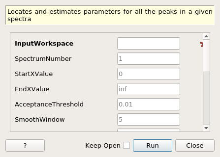
FindPeaksAutomatic dialog.
Table of Contents
| Name | Direction | Type | Default | Description |
|---|---|---|---|---|
| InputWorkspace | Input | Workspace | Mandatory | Workspace with peaks to be identified |
| SpectrumNumber | Input | number | 1 | Spectrum number to use |
| StartXValue | Input | number | 0 | Value of X to start the search from |
| EndXValue | Input | number | Optional | Value of X to stop the search to |
| AcceptanceThreshold | Input | number | 0.01 | Threshold for considering a peak significant, the exact meaning of the value depends on the cost function used and the data to be fitted. Good values might be about 1-10 for poisson cost and 0.0001-0.01 for chi2 |
| SmoothWindow | Input | number | 5 | Half size of the window used to find the background values to subtract |
| BadPeaksToConsider | Input | number | 20 | Number of peaks that do not exceed the acceptance threshold to be searched before terminating. This is useful because sometimes good peaks can be found after some bad ones. However setting this value too high will make the search much slower. |
| UsePoissonCost | Input | boolean | False | Use a probabilistic approach to find the cost of a fit instead of using chi2. |
| FitToBaseline | Input | boolean | False | Use a probabilistic approach to find the cost of a fit instead of using chi2. |
| EstimatePeakSigma | Input | number | 3 | A rough estimate of the standard deviation of the gaussian used to fit the peaks |
| MinPeakSigma | Input | number | 0.5 | Minimum value for the standard deviation of a peak |
| MaxPeakSigma | Input | number | 30 | Maximum value for the standard deviation of a peak |
| PlotPeaks | Input | boolean | False | Plot the position of the peaks found by the algorithm |
| PlotBaseline | Input | boolean | False | Plot the baseline as calculated by the algorithm |
| PeakPropertiesTableName | Output | TableWorkspace | peak_table | Name of the table containing the properties of the peaks |
| RefitPeakPropertiesTableName | Output | TableWorkspace | refit_peak_table | Name of the table containing the properties of the peaks that had to be fitted twice as the first time the error was unreasonably large |
| OutputWorkspace | Output | Workspace | workspace_with_errors | Workspace containing the same data as the input one, with errors added if not present from the beginning |
The algorithm takes a workspace containing a spectrum and will attempt to find the number and parameters of all the peaks (assumed to be gaussian).
To do so the algorithm performs the following:
To fit a list of peaks and calculate the cost algorithm FitGaussianPeaks is used. If the option PlotPeaks is selected then after completing the algorithm a plot of the input data is generated and the peaks marked with red x. If the option PlotBaseline is also selected then the baseline will also be shown. This is particularly useful when tuning the value of SmoothWindow (see below).
The result of the fit is strongly dependent on the parameter chosen. Unfortunately these depend on the particular data to be fitted. Therefore, while the default choice will often generate reasonable answers it is often necessary to adjust some of them.
The most important to this effect are:
Example - Find two gaussian peaks on an exponential background with added noise
# Function for a gaussian peak
def gaussian(xvals, centre, height, sigma):
    exp_val = (xvals - centre) / (np.sqrt(2) * sigma)

    return height * np.exp(-exp_val * exp_val)


np.random.seed(1234)

# Creating two peaks on an exponential background with gaussian noise
x_values = np.linspace(0, 1000, 1001)
centre = [250, 750]
height = [350, 200]
width = [3, 2]
y_values = gaussian(x_values, centre[0], height[0], width[0])
y_values += gaussian(x_values, centre[1], height[1], width[1])
y_values_low_noise = y_values + np.abs(400 * np.exp(-0.005 * x_values)) + 30 + 0.1*np.random.randn(len(x_values))
y_values_high_noise = y_values + np.abs(400 * np.exp(-0.005 * x_values)) + 30 + 10*np.random.randn(len(x_values))
low_noise_ws = CreateWorkspace(DataX=x_values, DataY=y_values_low_noise, DataE=np.sqrt(y_values_low_noise))
high_noise_ws = CreateWorkspace(DataX=x_values, DataY=y_values_high_noise, DataE=np.sqrt(y_values_high_noise))

# Fitting the data with low noise
FindPeaksAutomatic(InputWorkspace=low_noise_ws,
                  AcceptanceThreshold=0.2,
                  SmoothWindow=30,
                  EstimatePeakSigma=2,
                  MaxPeakSigma=5,
                  PlotPeaks=False,
                  PeakPropertiesTableName='properties',
                  RefitPeakPropertiesTableName='refit_properties')
peak_properties = mtd['properties']
peak_low1 = peak_properties.row(0)
peak_low2 = peak_properties.row(1)

# Fitting the data with strong noise
FindPeaksAutomatic(InputWorkspace=high_noise_ws,
                  AcceptanceThreshold=0.1,
                  SmoothWindow=30,
                  EstimatePeakSigma=2,
                  MaxPeakSigma=5,
                  PlotPeaks=False,
                  PeakPropertiesTableName='properties',
                  RefitPeakPropertiesTableName='refit_properties')
peak_properties = mtd['properties']
peak_high1 = peak_properties.row(0)
peak_high2 = peak_properties.row(1)

print('Low noise')
print('Peak 1: centre={:.2f}+/-{:.2f}, height={:.2f}+/-{:.2f}, sigma={:.2f}+/-{:.2f}'
      .format(peak_low1['centre'], peak_low1['error centre'],
              peak_low1['height'], peak_low1['error height'],
              peak_low1['sigma'], peak_low1['error sigma']))
print('Peak 2: centre={:.2f}+/-{:.2f}, height={:.2f}+/-{:.2f}, sigma={:.2f}+/-{:.2f}'
      .format(peak_low2['centre'], peak_low2['error centre'],
              peak_low2['height'], peak_low2['error height'],
              peak_low2['sigma'], peak_low2['error sigma']))
print('')

print('Strong noise')
print('Peak 1: centre={:.2f}+/-{:.2f}, height={:.2f}+/-{:.2f}, sigma={:.2f}+/-{:.2f}'
      .format(peak_high1['centre'], peak_high1['error centre'],
              peak_high1['height'], peak_high1['error height'],
              peak_high1['sigma'], peak_high1['error sigma']))
print('Peak 2: centre={:.2f}+/-{:.2f}, height={:.2f}+/-{:.2f}, sigma={:.2f}+/-{:.2f}'
      .format(peak_high2['centre'], peak_high2['error centre'],
              peak_high2['height'], peak_high2['error height'],
              peak_high2['sigma'], peak_high2['error sigma']))
Output:
Low noise
Peak 1: centre=250.01+/-0.09, height=352.47+/-10.91, sigma=3.06+/-0.08
Peak 2: centre=750.00+/-0.09, height=200.03+/-9.13, sigma=2.01+/-0.07

Strong noise
Peak 1: centre=250.00+/-0.09, height=360.33+/-10.83, sigma=3.11+/-0.08
Peak 2: centre=749.90+/-0.08, height=194.86+/-7.82, sigma=2.47+/-0.07
Example - Find 2 different gaussian peaks on a flat background with added noise
    # Function for a gaussian peak
def gaussian(xvals, centre, height, sigma):
    exp_val = (xvals - centre) / (np.sqrt(2) * sigma)

    return height * np.exp(-exp_val * exp_val)


np.random.seed(4321)

# Creating two peaks on a flat background with gaussian noise
x_values = np.array([np.linspace(0, 1000, 1001), np.linspace(0, 1000, 1001)], dtype=float)
centre = np.array([[250, 750], [100, 600]], dtype=float)
height = np.array([[350, 200], [400, 500]], dtype=float)
width = np.array([[10, 5], [3, 2]], dtype=float)
y_values = np.array([gaussian(x_values[0], centre[0, 0], height[0, 0], width[0, 0]),
                     gaussian(x_values[1], centre[1, 0], height[1, 0], width[1, 0])])
y_values += np.array([gaussian(x_values[0], centre[0, 1], height[0, 1], width[0, 1]),
                      gaussian(x_values[1], centre[1, 1], height[1, 1], width[1, 1])])
y_values_low_noise = y_values + np.abs(200 + 0.1*np.random.randn(*x_values.shape))
y_values_high_noise = y_values + np.abs(200 + 5*np.random.randn(*x_values.shape))
low_noise_ws = CreateWorkspace(DataX=x_values, DataY=y_values_low_noise, DataE=np.sqrt(y_values_low_noise),NSpec = 2)
high_noise_ws = CreateWorkspace(DataX=x_values, DataY=y_values_high_noise, DataE=np.sqrt(y_values_high_noise),NSpec =2)

# Fitting the data with low noise
FindPeaksAutomatic(InputWorkspace=low_noise_ws,
                  SpectrumNumber = 2,
                  AcceptanceThreshold=0.2,
                  SmoothWindow=30,
                  EstimatePeakSigma=2,
                  MaxPeakSigma=5,
                  PlotPeaks=False,
                  PeakPropertiesTableName='properties',
                  RefitPeakPropertiesTableName='refit_properties')
peak_properties = mtd['properties']
peak_low1 = peak_properties.row(0)
peak_low2 = peak_properties.row(1)

# Fitting the data with strong noise
FindPeaksAutomatic(InputWorkspace=high_noise_ws,
                  SpectrumNumber = 2,
                  AcceptanceThreshold=0.1,
                  SmoothWindow=30,
                  EstimatePeakSigma=2,
                  MaxPeakSigma=5,
                  PlotPeaks=False,
                  PeakPropertiesTableName='properties',
                  RefitPeakPropertiesTableName='refit_properties')
peak_properties = mtd['properties']
peak_high1 = peak_properties.row(0)
peak_high2 = peak_properties.row(1)

print('Low noise')
print('Peak 1: centre={:.2f}+/-{:.2f}, height={:.2f}+/-{:.2f}, sigma={:.2f}+/-{:.2f}'
      .format(peak_low1['centre'], peak_low1['error centre'],
              peak_low1['height'], peak_low1['error height'],
              peak_low1['sigma'], peak_low1['error sigma']))
print('Peak 2: centre={:.2f}+/-{:.2f}, height={:.2f}+/-{:.2f}, sigma={:.2f}+/-{:.2f}'
      .format(peak_low2['centre'], peak_low2['error centre'],
              peak_low2['height'], peak_low2['error height'],
              peak_low2['sigma'], peak_low2['error sigma']))
print('')

print('Strong noise')
print('Peak 1: centre={:.2f}+/-{:.2f}, height={:.2f}+/-{:.2f}, sigma={:.2f}+/-{:.2f}'
      .format(peak_high1['centre'], peak_high1['error centre'],
              peak_high1['height'], peak_high1['error height'],
              peak_high1['sigma'], peak_high1['error sigma']))
print('Peak 2: centre={:.2f}+/-{:.2f}, height={:.2f}+/-{:.2f}, sigma={:.2f}+/-{:.2f}'
      .format(peak_high2['centre'], peak_high2['error centre'],
              peak_high2['height'], peak_high2['error height'],
              peak_high2['sigma'], peak_high2['error sigma']))
Output:
Low noise
Peak 1: centre=100.00+/-0.09, height=400.19+/-12.18, sigma=3.00+/-0.08
Peak 2: centre=600.00+/-0.06, height=500.20+/-16.01, sigma=2.00+/-0.06

Strong noise
Peak 1: centre=100.00+/-0.10, height=377.97+/-0.02, sigma=3.35+/-0.07
Peak 2: centre=600.00+/-0.06, height=503.59+/-15.68, sigma=2.08+/-0.06
Categories: AlgorithmIndex | Optimization\PeakFinding
Python: FindPeaksAutomatic.py