\(\renewcommand\AA{\unicode{x212B}}\)
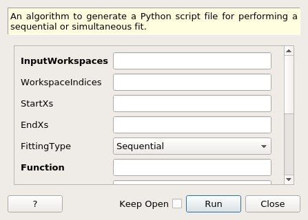
GeneratePythonFitScript dialog.
Table of Contents
An algorithm to generate a Python script file for performing a sequential or simultaneous fit.
| Name | Direction | Type | Default | Description |
|---|---|---|---|---|
| InputWorkspaces | Input | str list | Mandatory | A list of workspace names to be fitted. The workspace name at index i in the list corresponds with the ‘WorkspaceIndices’, ‘StartXs’ and ‘EndXs’ properties. |
| WorkspaceIndices | Input | unsigned int list | A list of workspace indices to be fitted. The workspace index at index i in the list will correspond to the input workspace at index i. | |
| StartXs | Input | dbl list | A list of start X’s to be used for the fitting. The Start X at index i will correspond to the input workspace at index i. | |
| EndXs | Input | dbl list | A list of end X’s to be used for the fitting. The End X at index i will correspond to the input workspace at index i. | |
| FittingType | Input | string | Sequential | The type of fitting to generate a python script for (Sequential or Simultaneous). Allowed values: [‘Sequential’, ‘Simultaneous’] |
| Function | Input | Function | Mandatory | The function to use for the fitting. This should be a single domain function if the Python script will be for sequential fitting, or a MultiDomainFunction if the Python script is for simultaneous fitting. |
| MaxIterations | Input | number | 500 | The MaxIterations to be passed to the Fit algorithm in the Python script. |
| Minimizer | Input | string | Levenberg-Marquardt | The Minimizer to be passed to the Fit algorithm in the Python script. Allowed values: [‘BFGS’, ‘Conjugate gradient (Fletcher-Reeves imp.)’, ‘Conjugate gradient (Polak-Ribiere imp.)’, ‘Damped GaussNewton’, ‘FABADA’, ‘Levenberg-Marquardt’, ‘Levenberg-MarquardtMD’, ‘Simplex’, ‘SteepestDescent’, ‘Trust Region’] |
| CostFunction | Input | string | Least squares | The CostFunction to be passed to the Fit algorithm in the Python script. Allowed values: [‘Least squares’, ‘Poisson’, ‘Rwp’, ‘Unweighted least squares’] |
| EvaluationType | Input | string | CentrePoint | The EvaluationType to be passed to the Fit algorithm in the Python script. Allowed values: [‘CentrePoint’, ‘Histogram’] |
| OutputBaseName | Input | string | Output_Fit | The OutputBaseName is the base output name to use for the resulting Fit workspaces. |
| PlotOutput | Input | boolean | True | If true, code used for plotting the results of a fit will be generated and added to the python script. |
| Filepath | Input | string | The name of the Python fit script which will be generated and saved in the selected location. Allowed extensions: [‘.py’] | |
| ScriptText | Output | string |
This algorithm can be used to generate a python script used for sequential or simultaneous fitting. The generated python script is intended to be a generic example for how you can perform a fit in Mantid, and can easily be adapted for specific needs. This algorithm is used by the Fit Script Generator interface.
Example - generate a python script used for sequential fitting:
ws1 = CreateSampleWorkspace()
ws2 = CreateSampleWorkspace()

function = \
"name=GausOsc,A=0.2,Sigma=0.2,Frequency=1,Phi=0"

# If you want to save the python script to a file then specify the Filepath property
script_text = GeneratePythonFitScript(InputWorkspaces=["ws1", "ws1", "ws2", "ws2"], WorkspaceIndices=[0, 1, 0, 1],
                                      StartXs=[0.0, 0.0, 0.0, 0.0], EndXs=[20000.0, 20000.0, 20000.0, 20000.0],
                                      FittingType="Sequential", Function=function, MaxIterations=500,
                                      Minimizer="Levenberg-Marquardt", OutputBaseName="Output_Fit")

print(script_text)
Output:
# A python script generated to perform a sequential or simultaneous fit
from mantid.simpleapi import *
import matplotlib.pyplot as plt

# Dictionary { workspace_name: (workspace_index, start_x, end_x) }
input_data = {
    "ws1": (0, 0.000000, 20000.000000),
    "ws1": (1, 0.000000, 20000.000000),
    "ws2": (0, 0.000000, 20000.000000),
    "ws2": (1, 0.000000, 20000.000000)
}

# Fit function as a string
function = \
    "name=GausOsc,A=0.2,Sigma=0.2,Frequency=1,Phi=0"

# Fitting options
max_iterations = 500
minimizer = "Levenberg-Marquardt"
cost_function = "Least squares"
evaluation_type = "CentrePoint"
output_base_name = "Output_Fit"

# Perform a sequential fit
output_workspaces, parameter_tables, normalised_matrices = [], [], []
for input_workspace, domain_data in input_data.items():
    fit_output = Fit(Function=function, InputWorkspace=input_workspace, WorkspaceIndex=domain_data[0],
                     StartX=domain_data[1], EndX=domain_data[2], MaxIterations=max_iterations,
                     Minimizer=minimizer, CostFunction=cost_function, EvaluationType=evaluation_type,
                     Output=output_base_name + input_workspace)

    output_workspaces.append(output_base_name + input_workspace + "_Workspace")
    parameter_tables.append(output_base_name + input_workspace + "_Parameters")
    normalised_matrices.append(output_base_name + input_workspace + "_NormalisedCovarianceMatrix")

    # Use the parameters in the previous function as the start parameters of the next fit
    function = fit_output.Function

# Group the output workspaces from the sequential fit
GroupWorkspaces(InputWorkspaces=output_workspaces, OutputWorkspace=output_base_name + "Workspaces")
GroupWorkspaces(InputWorkspaces=parameter_tables, OutputWorkspace=output_base_name + "Parameters")
GroupWorkspaces(InputWorkspaces=normalised_matrices, OutputWorkspace=output_base_name + "NormalisedCovarianceMatrices")

# Plot the results of the fit
fig, axes = plt.subplots(nrows=2,
                         ncols=len(output_workspaces),
                         sharex=True,
                         gridspec_kw={"height_ratios": [2, 1]},
                         subplot_kw={"projection": "mantid"})

for i, workspace_name in enumerate(output_workspaces):
    workspace = AnalysisDataService.retrieve(workspace_name)
    axes[0, i].errorbar(workspace, "rs", wkspIndex=0, label="Data", markersize=2)
    axes[0, i].errorbar(workspace, "b-", wkspIndex=1, label="Fit")
    axes[0, i].set_title(workspace_name)
    axes[0, i].set_xlabel("")
    axes[0, i].tick_params(axis="both", direction="in")
    axes[0, i].legend()

    axes[1, i].errorbar(workspace, "ko", wkspIndex=2, markersize=2)
    axes[1, i].set_ylabel("Difference")
    axes[1, i].tick_params(axis="both", direction="in")

fig.subplots_adjust(hspace=0)
fig.show()
Example - generate a python script used for simultaneous fitting:
ws1 = CreateSampleWorkspace()
ws2 = CreateSampleWorkspace()

function = \
"composite=MultiDomainFunction,NumDeriv=true;" \
"name=GausOsc,A=0.2,Sigma=0.2,Frequency=1,Phi=0,$domains=i;" \
"name=GausOsc,A=0.2,Sigma=0.2,Frequency=1,Phi=0,$domains=i;" \
"name=GausOsc,A=0.2,Sigma=0.2,Frequency=1,Phi=0,$domains=i;" \
"name=GausOsc,A=0.2,Sigma=0.2,Frequency=1,Phi=0,$domains=i;" \
"ties=(f2.Frequency=f3.Frequency,f1.Frequency=f3.Frequency,f0.Frequency=f3.Frequency)"

# If you want to save the python script to a file then specify the Filepath property
script_text = GeneratePythonFitScript(InputWorkspaces=["ws1", "ws1", "ws2", "ws2"], WorkspaceIndices=[0, 1, 0, 1],
                                      StartXs=[0.0, 0.0, 0.0, 0.0], EndXs=[20000.0, 20000.0, 20000.0, 20000.0],
                                      FittingType="Simultaneous", Function=function, MaxIterations=500,
                                      Minimizer="Levenberg-Marquardt", OutputBaseName="Output_Fit")

print(script_text)
Output:
# A python script generated to perform a sequential or simultaneous fit
from mantid.simpleapi import *
import matplotlib.pyplot as plt

# Dictionary { workspace_name: (workspace_index, start_x, end_x) }
input_data = {
    "ws1": (0, 0.000000, 20000.000000),
    "ws1": (1, 0.000000, 20000.000000),
    "ws2": (0, 0.000000, 20000.000000),
    "ws2": (1, 0.000000, 20000.000000)
}

# Fit function as a string
function = \
    "composite=MultiDomainFunction,NumDeriv=true;" \
    "name=GausOsc,A=0.2,Sigma=0.2,Frequency=1,Phi=0,$domains=i;" \
    "name=GausOsc,A=0.2,Sigma=0.2,Frequency=1,Phi=0,$domains=i;" \
    "name=GausOsc,A=0.2,Sigma=0.2,Frequency=1,Phi=0,$domains=i;" \
    "name=GausOsc,A=0.2,Sigma=0.2,Frequency=1,Phi=0,$domains=i;" \
    "ties=(f2.Frequency=f3.Frequency,f1.Frequency=f3.Frequency,f0.Frequency=f3.Frequency)"

# Fitting options
max_iterations = 500
minimizer = "Levenberg-Marquardt"
cost_function = "Least squares"
evaluation_type = "CentrePoint"
output_base_name = "Output_Fit"

# Perform a simultaneous fit
input_workspaces = list(input_data.keys())
domain_data = list(input_data.values())

fit_output = \
    Fit(Function=function,
        InputWorkspace=input_workspaces[0], WorkspaceIndex=domain_data[0][0], StartX=domain_data[0][1], EndX=domain_data[0][2],
        InputWorkspace_1=input_workspaces[1], WorkspaceIndex_1=domain_data[1][0], StartX_1=domain_data[1][1], EndX_1=domain_data[1][2],
        InputWorkspace_2=input_workspaces[2], WorkspaceIndex_2=domain_data[2][0], StartX_2=domain_data[2][1], EndX_2=domain_data[2][2],
        InputWorkspace_3=input_workspaces[3], WorkspaceIndex_3=domain_data[3][0], StartX_3=domain_data[3][1], EndX_3=domain_data[3][2],
        MaxIterations=max_iterations, Minimizer=minimizer, CostFunction=cost_function,
        EvaluationType=evaluation_type, Output=output_base_name)

output_workspaces = []
for i in range(len(input_workspaces)):
    output_workspaces.append(output_base_name + "_Workspace_" + str(i))

# Plot the results of the fit
fig, axes = plt.subplots(nrows=2,
                         ncols=len(output_workspaces),
                         sharex=True,
                         gridspec_kw={"height_ratios": [2, 1]},
                         subplot_kw={"projection": "mantid"})

for i, workspace_name in enumerate(output_workspaces):
    workspace = AnalysisDataService.retrieve(workspace_name)
    axes[0, i].errorbar(workspace, "rs", wkspIndex=0, label="Data", markersize=2)
    axes[0, i].errorbar(workspace, "b-", wkspIndex=1, label="Fit")
    axes[0, i].set_title(workspace_name)
    axes[0, i].set_xlabel("")
    axes[0, i].tick_params(axis="both", direction="in")
    axes[0, i].legend()

    axes[1, i].errorbar(workspace, "ko", wkspIndex=2, markersize=2)
    axes[1, i].set_ylabel("Difference")
    axes[1, i].tick_params(axis="both", direction="in")

fig.subplots_adjust(hspace=0)
fig.show()
Categories: AlgorithmIndex | Utility\Python