\(\renewcommand\AA{\unicode{x212B}}\)
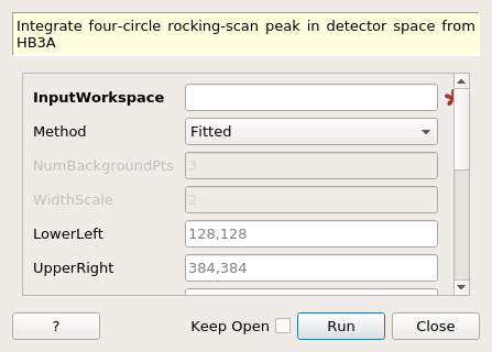
HB3AIntegrateDetectorPeaks dialog.
Table of Contents
| Name | Direction | Type | Default | Description |
|---|---|---|---|---|
| InputWorkspace | Input | str list | Mandatory | Workspace or comma-separated workspace list containing input MDHisto scan data. |
| Method | Input | string | Fitted | Integration method to use. Allowed values: [‘Counts’, ‘CountsWithFitting’, ‘Fitted’] |
| NumBackgroundPts | Input | number | 3 | Number of background points from beginning and end of scan to use for background estimation |
| WidthScale | Input | number | 2 | Controls integration range (+/- WidthScale/2*FWHM) defined around motor positions for CountsWithFitting method |
| LowerLeft | Input | long list | 128,128 | Region of interest lower-left corner, in detector pixels |
| UpperRight | Input | long list | 384,384 | Region of interest upper-right corner, in detector pixels |
| StartX | Input | number | Optional | The start of the scan axis fitting range in degrees, either omega or chi axis. |
| EndX | Input | number | Optional | The end of the scan axis fitting range in degrees, either omega or chi axis. |
| ScaleFactor | Input | number | 1 | scale the integrated intensity by this value |
| ChiSqMax | Input | number | 10 | Fitting resulting in chi-sqaured higher than this won’t be added to the output |
| SignalNoiseMin | Input | number | 1 | Minimum Signal/Noice ratio (Intensity/SigmaIntensity) of peak to be added to the output |
| ApplyLorentz | Input | boolean | True | If to apply Lorentz Correction to intensity |
| OutputFitResults | Input | boolean | False | This will output the fitting result workspace and a ROI workspace |
| OptimizeQVector | Input | boolean | True | This will convert the data to q and optimize the peak location using CentroidPeaksdMD |
| OutputWorkspace | Output | IPeaksWorkspace | Mandatory | Output Peaks Workspace |
The input to this algorithm is intended as part of the DEMAND data reduction workflow, using HB3AAdjustSampleNorm with OutputType=Detector which can be seen below in the example usage.
This will reduce the input workspace using the region of interest provided to create a 1-dimension workspace with an axis that is the detector scan, either omega or chi in degrees.
An optional fitting range of the scan axis can be provided with StartX and EndX in degrees, which is applicable for the CountsWithFitting and Fitted methods.
The OptimizeQVector option will convert the input data into Q and use CentroidPeaksdMD to find the correct Q-vector starting from the known HKL and UB matrix of the peaks. This will not effect the integration of the peak but allows the UB matrix to be refined afterwards.
There are three different methods for integrating the input workspace: simple counts summation, simple counts summation with fitted background, and a fitted model.
This method uses the simple cuboid integration to approximate the integrated peak intensity.
The error is calculated as
The background is estimated by averaging data from the first and last scans:
where \(<pt>\) is the number of scans to include in the background estimation and is specified with the NumBackgroundPts option.
For Method=CountsWithFitting, the input is fit to a Gaussian with a flat background, just like Method=Fitting. However, the peak intensity is instead approximated by summing the detector counts over a specific set of measurements that are defined by the motor positions in the range of \(\pm \frac{N}{2} \text{FWHM}\), where N is controlled with the WidthScale option. The background is removed over the same range using the fitted flat background.
The error is calculated as
For Method=Fitted, the reduced workspace is fitted using Fit with a flat background and a Gaussian, then the area of the Gaussian is used as the peak intensity:
The error of the intensity is calculated by the propagation of fitted error of A and s.
Example - DEMAND single detector peak integration
data = HB3AAdjustSampleNorm(Filename='HB3A_data.nxs', OutputType='Detector')
peaks = HB3AIntegrateDetectorPeaks(data,
                                   ChiSqMax=100,
                                   OutputFitResults=True,
                                   LowerLeft=[200, 200],
                                   UpperRight=[312, 312])
print('HKL={h:.0f}{k:.0f}{l:.0f} λ={Wavelength}Å Intensity={Intens:.3f}'.format(**peaks.row(0)))
HKL=006 λ=1.008Å Intensity=211.753
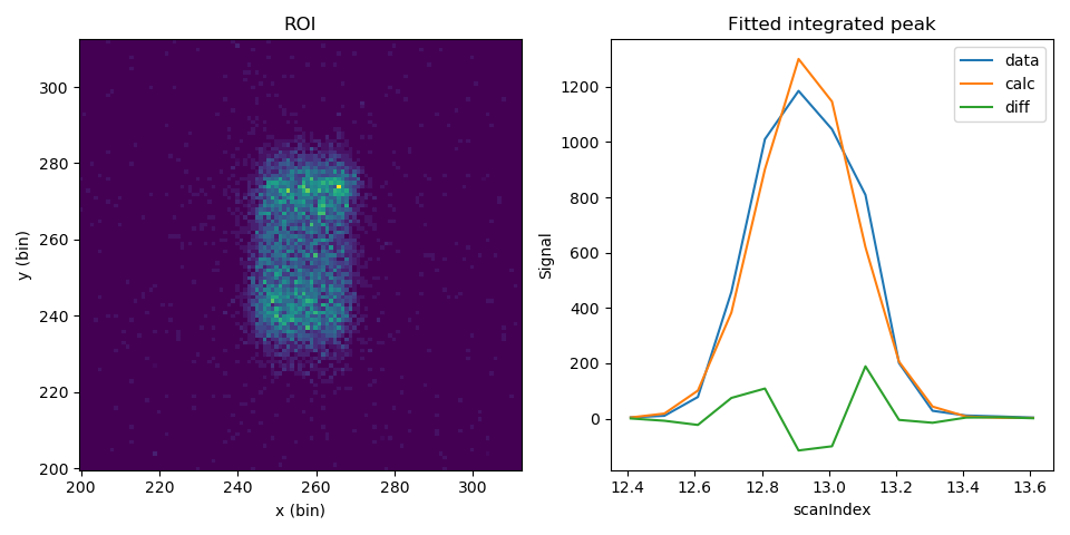
To check the ROI and peak fitting you can plot the results
import matplotlib.pyplot as plt
fig = plt.figure(figsize=(9.6, 4.8))
ax1 = fig.add_subplot(121, projection='mantid')
ax2 = fig.add_subplot(122, projection='mantid')
ax1.pcolormesh(mtd['peaks_data_ROI'], transpose=True)
ax1.set_title("ROI")
ax2.plot(mtd['peaks_data_Workspace'], wkspIndex=0, label='data')
ax2.plot(mtd['peaks_data_Workspace'], wkspIndex=1, label='calc')
ax2.plot(mtd['peaks_data_Workspace'], wkspIndex=2, label='diff')
ax2.legend()
ax2.set_title("Fitted integrated peak")
fig.tight_layout()
fig.show()
Example - DEMAND multiple files, indexing with modulation vector
IPTS = 24855
exp = 755
scans = range(28, 96)
filename = '/HFIR/HB3A/IPTS-{}/shared/autoreduce/HB3A_exp{:04}_scan{:04}.nxs'

data = HB3AAdjustSampleNorm(','.join(filename.format(IPTS, exp, scan) for scan in scans), OutputType="Detector")
peaks = HB3AIntegrateDetectorPeaks(data)
IndexPeaks(peaks, ModVector1='0,0,0.5', MaxOrder=1, SaveModulationInfo=True)
SaveReflections(peaks, Filename='peaks.hkl')
Categories: AlgorithmIndex | Crystal\Integration
Python: HB3AIntegrateDetectorPeaks.py