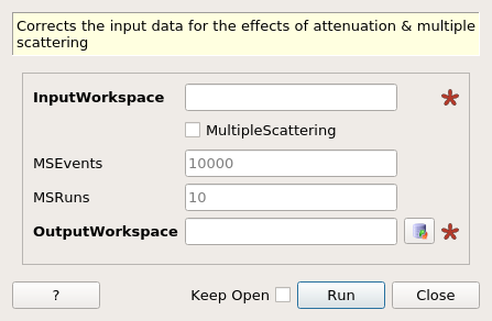
MayersSampleCorrection v1¶

Summary¶

Corrects the input data for the effects of attenuation & multiple scattering

Properties¶

Description¶

Calculates and applies corrections due to the effects of absorption (plus optionally multiple scattering) on the signal and error values for a given workspace. The full background to the algorithm is described by Lindley et al. [1] and is briefly described here.

The following assumptions are made:

• the sample shape is a cylinder

• for multiple scattering:

  • the scattering is assumed to be elastic and isotropic
  • the ratio of successive orders of scattering are all equal to \(\beta(\theta, \phi, E)\)

The aim is to correct the number of neutrons at a given detector (\(N_d\)) to compute the number of neutrons (\(N_c\)) that would reach the detector if there was no absorption (or multiple scattering). Ignoring detector efficiency we can write:

where \(A_s(\theta, \phi, E)\) is the absorption and self-shielding factor and is computed by numerical integration over the sample cylinder.

The multiple scattering factor (if requested) is computed by simulating over a fixed number of second order scattering events and computing the ratio of second order and first order scattering. Since we have assumed the ratio is the same between successive orders, the \(\frac{1}{1-\beta}\) factor simply comes from taking the sum of a geometric series.

The cylinder radius \(r\) combined with the inverse attenuation length \(\mu = \mu(E)\) (derived from the total scattering cross-section) gives a range of \(\mu r\) against input time-of-flight (“energy”) for the cylinder. The \(\mu r\) range is divided into a discrete number of points for each point.

A weighted least-squares fit is applied to both the set of attenuation and multiple scattering factors to allow interpolation of the correction factor from any time-of-flight value in the input range. For each time-of-flight value the factor is computed from the fit coefficients and the correction applied multiplicatively:

The above procedure is repeated separately for each spectrum in the workspace.

Usage¶

Example - Correct Vanadium For Both Absorption & Multiple Scattering

# Create a fake workspace with TOF data
sample_ws = CreateSampleWorkspace(Function='Powder Diffraction',
                                  NumBanks=1,BankPixelWidth=1,XUnit='TOF',
                                  XMin=1000,XMax=10000)
# Set meta data about shape and material
cyl_height_cm = 4.0
cyl_radius_cm = 0.25
material = 'V'
num_density = 0.07261
SetSample(sample_ws,
    Geometry={'Shape': 'Cylinder', 'Height': cyl_height_cm,
              'Radius': cyl_radius_cm, 'Center': [0.0,0.0,0.0]},
    Material={'ChemicalFormula': material, 'SampleNumberDensity': num_density})

# Run corrections
corrected_sample = MayersSampleCorrection(sample_ws,
                                          MultipleScattering=True)

# Print a bin
print("Uncorrected signal: {0:.4f}".format(sample_ws.readY(0)[25]))
print("Corrected signal: {0:.4f}".format(corrected_sample.readY(0)[25]))

Output:

Uncorrected signal: 0.0556
Corrected signal: 0.0736

References¶

Categories: AlgorithmIndex | CorrectionFunctions\AbsorptionCorrections

Source¶

C++ header: MayersSampleCorrection.h

C++ source: MayersSampleCorrection.cpp