\(\renewcommand\AA{\unicode{x212B}}\)
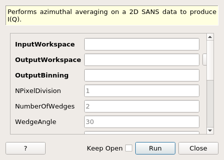
Q1DWeighted dialog.
Table of Contents
| Name | Direction | Type | Default | Description |
|---|---|---|---|---|
| InputWorkspace | Input | MatrixWorkspace | Mandatory | Input workspace containing the SANS 2D data |
| OutputWorkspace | Output | MatrixWorkspace | Mandatory | Workspace that will contain the I(Q) data |
| OutputBinning | Input | dbl list | Mandatory | The new bin boundaries in the form: \(x_1,\Delta x_1,x_2,\Delta x_2,\dots,x_n\) |
| NPixelDivision | Input | number | 1 | Number of sub-pixels used for each detector pixel in each direction.The total number of sub-pixels will be NPixelDivision*NPixelDivision. |
| NumberOfWedges | Input | number | 2 | Number of wedges to calculate. |
| WedgeAngle | Input | number | 30 | Opening angle of the wedge, in degrees. |
| WedgeOffset | Input | number | 0 | Wedge offset relative to the horizontal axis, in degrees. |
| WedgeWorkspace | Output | WorkspaceGroup | Name for the WorkspaceGroup containing the wedge I(q) distributions. | |
| PixelSizeX | Input | number | 5.15 | Pixel size in the X direction (mm). |
| PixelSizeY | Input | number | 5.15 | Pixel size in the Y direction (mm). |
| ErrorWeighting | Input | boolean | False | Choose whether each pixel contribution will be weighted by 1/error^2. |
| AsymmetricWedges | Input | boolean | False | Choose to produce the results for asymmetric wedges. |
| AccountForGravity | Input | boolean | False | Take the nominal gravity drop into account. |
| ShapeTable | Input | TableWorkspace | Table workspace containing the shapes (sectors only) drawn in the instrument viewer; if specified, the wedges properties defined above are not taken into account. |
Performs azimuthal averaging for a 2D SANS data set by going through each wavelength bin of each detector pixel, determining its Q-value, and adding its amplitude \(I\) to the appropriate Q bin. The algorithm works both for monochromatic and TOF SANS data.
Note that in TOF case, the algorithm performs averaging in 2 steps.
First, for each wavelength slice of the input it performs azimuthal averaging in radial rings.
This results in a stack of I(Q)s, one for each input wavelength.
As a second step, all the I(Q)s corresponding to different wavelengths are averaged again.
Note that for the TOF data, this is mathematically not equivalent to performing averaging with one step; that is averaging everything into a single I(Q) histogram.
The latter is done in Q1D algorithm.
See the Rebin documentation for details about choosing the OutputBinning parameter.
For monochromatic data, the algorithm considers each bin as belonging to a different sample and/or kinetic frame. Usage —–
This algorithm is used as a part of the SANSReduction and SANSILLIntegration. However, it can also be used directly, provided that the input data is already corrected for all the effects.
The input to this algorithm must be a histogram with common wavelength bins for each pixel, or a monochromatic workspace with a different sample or kinetic frame in each bin. In this case the workspace must not be in units of wavelength, but the wavelength must be present in the sample logs. The output will be a distribution though.
For greater precision, each detector
pixel can be sub-divided in sub-pixels by setting the NPixelDivision
parameters. This will split each pixel to a grid of NPixelDivision * NPixelDivision pixels.
PixelSizeX and PixelSizeY inputs will be used only if pixels are to be split.
Each pixel has a weight of 1 by default, but the weight of
each pixel can be set to \(1/\sigma^2 I\) by setting the
ErrorWeighting parameter to True. This will effectively transmute the average to a weighted average, where the weight is inversely proportional to the absolute statistical uncertainty on the intensity.
This option will potentially produce very different results, so care must be taken when analysing the data with this option.
In the reduction workflows this option is deprecated.
For anisotropic scatterer, the I(Q) can be calculated for different angular sectors (or wedges).
These sectors can be defined in two different ways : either by drawing them, or by defining them. There are also two integration mode: symmetric wedges (default) or asymmetric wedges.
Wedges are defined by the NumberOfWedges, WedgeAngle and WedgeOffset parameters.
The trigonometrical circle is split in NumberOfWedges sectors, equally spaced, spanning a range of WedgeAngle.
This option is still in active development, and might be subject to changes in later versions.
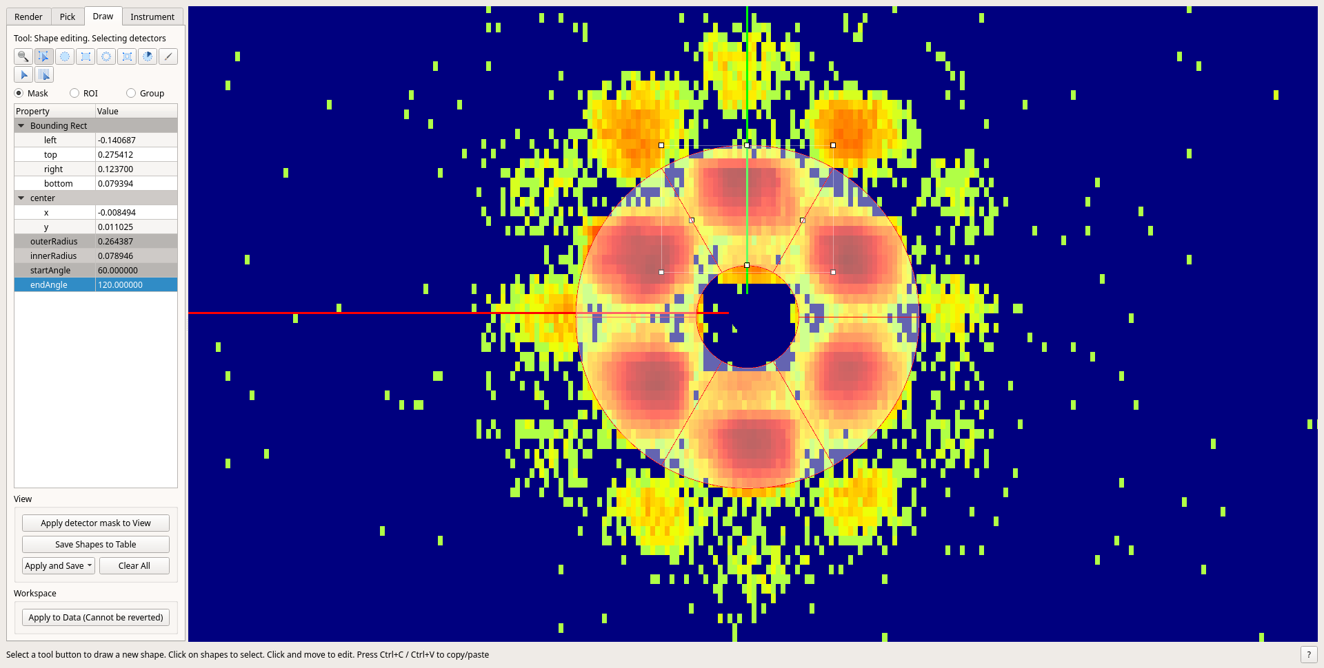
It is also possible to use the instrument viewer to draw the shape of the angular sector. Only sector shapes are currently supported,
and they must be drawn in the Full 3D, Z- projection, without any rotation (translation and zoom are supported). Please
note that in this projection, the X-axis points to the left. So when doing the wedges without the table (see above), they are ordered
clockwise, opening from the positive ray of the X-axis.
If running Q1DWeighted with drawn sectors as input, the output will be ordered similarly, regardless of the order in which they were drawn.
Once the shapes are drawn, they must be saved using the Save shapes to table button.
Contrary to the wedges defined in the previous manner, the sectors don’t need to be regularly placed, centered or even symmetrical.
When running Q1DWeighted, the created table workspace - generally named MaskShapes - can be provided
as an argument to the ShapeTable field. The algorithm will then use the drawn shapes as wedges, and ignore NumberOfWedges,
WedgeAngle and WedgeOffset fields.
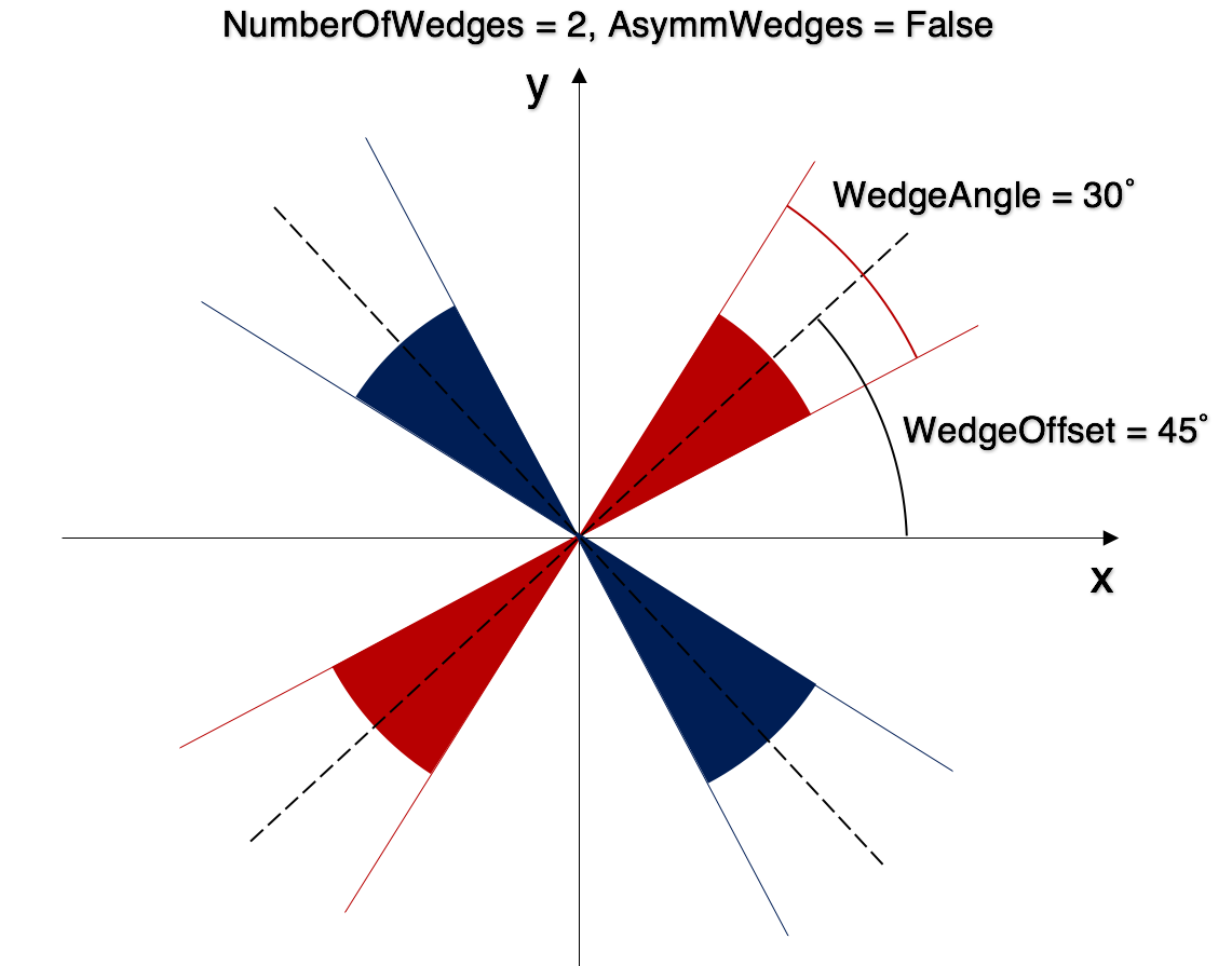
Symmetric or asymmetric integration is determined by the AsymmetricWedges flag.
The figure below illustrates an example for symmetric wedges. Each wedge in this case represents two back-to-back sectors. The wedges output group will have two workspaces: one for the red region, one for the blue region.
In the case of drawn sectors, when doing symmetric integration, symmetric shapes will be grouped together. Taking the above example, the shape table will have 4 shapes in it, but the output will only have 2 workspaces, because the red shapes and the blue shapes will be grouped. If no corresponding symmetric is found for a shape, the algorithm will nonetheless integrate on the projected symmetric too, so the result will be identical (though for clarity it is not advised to provide only one of the shapes). Again, in the above example, the result will be identical whether only one or both of the red and blue shapes are provided, because the algorithm will find the missing symmetric if needed.
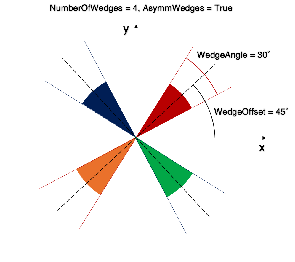
An example for asymmetric wedges is shown below. The output will have four workspaces, one per each sector of different color.
Bins masked in the input workspace will not enter the calculation.
If enabled, this will correct for the gravity effect by analytical calculation of the drop during the time-of-flight from sample to detector.
Categories: AlgorithmIndex | SANS