\(\renewcommand\AA{\unicode{x212B}}\)
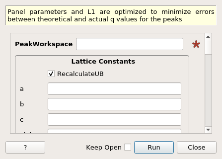
SCDCalibratePanels dialog.
Table of Contents
Panel parameters and L1 are optimized to minimize errors between theoretical and actual q values for the peaks
| Name | Direction | Type | Default | Description |
|---|---|---|---|---|
| PeakWorkspace | Input | IPeaksWorkspace | Mandatory | Workspace of Indexed Peaks |
| RecalculateUB | Input | boolean | True | Recalculate UB matrix using given lattice constants |
| a | Input | number | Optional | Lattice Parameter a (Leave empty to use lattice constants in peaks workspace) |
| b | Input | number | Optional | Lattice Parameter b (Leave empty to use lattice constants in peaks workspace) |
| c | Input | number | Optional | Lattice Parameter c (Leave empty to use lattice constants in peaks workspace) |
| alpha | Input | number | Optional | Lattice Parameter alpha in degrees (Leave empty to use lattice constants in peaks workspace) |
| beta | Input | number | Optional | Lattice Parameter beta in degrees (Leave empty to use lattice constants in peaks workspace) |
| gamma | Input | number | Optional | Lattice Parameter gamma in degrees (Leave empty to use lattice constants in peaks workspace) |
| CalibrateL1 | Input | boolean | True | Change the L1(source to sample) distance |
| SearchRadiusL1 | Input | number | 0.1 | Search radius of delta L1 in meters, which is used to constrain optimization search spacewhen calibrating L1 |
| CalibrateBanks | Input | boolean | False | Calibrate position and orientation of each bank. |
| SearchRadiusTransBank | Input | number | 0.05 | This is the search radius (in meter) when calibrating component translations, used to constrain optimizationsearch space when calibration translation of banks |
| SearchradiusRotXBank | Input | number | 1 | This is the search radius (in deg) when calibrating component reorientation, used to constrain optimization search space |
| SearchradiusRotYBank | Input | number | 1 | This is the search radius (in deg) when calibrating component reorientation, used to constrain optimization search space |
| SearchradiusRotZBank | Input | number | 1 | This is the search radius (in deg) when calibrating component reorientation, used to constrain optimization search space |
| CalibrateSize | Input | boolean | False | Calibrate detector size for each bank. |
| SearchRadiusSize | Input | number | 0 | This is the search radius (unit less) of scale factor around at value 1.0 when calibrating component size if it is a rectangualr detector. |
| FixAspectRatio | Input | boolean | True | If true, the scaling factor for detector along X- and Y-axis must be the same. Otherwise, the 2 scaling factors are free. |
| BankName | Input | string | If given, only the specified bank/component will be calibrated.Otherwise, all banks will be calibrated. | |
| CalibrateT0 | Input | boolean | False | Calibrate the T0 (initial TOF) |
| SearchRadiusT0 | Input | number | 10 | Search radius of T0 (in ms), used to constrain optimization search space |
| TuneSamplePosition | Input | boolean | False | Fine tunning sample position |
| SearchRadiusSamplePos | Input | number | 0.1 | Search radius of sample position change (in meters), used to constrain optimization search space |
| OutputWorkspace | Output | TableWorkspace | Mandatory | The workspace containing the calibration table. |
| T0 | Output | number | Returns the TOF offset from optimization | |
| DetCalFilename | Input | string | SCDCalibrate2.DetCal | Path to an ISAW-style .detcal file to save. Allowed extensions: [‘.detcal’, ‘.det_cal’] |
| XmlFilename | Input | string | SCDCalibrate2.xml | Path to an Mantid .xml description(for LoadParameterFile) file to save. Allowed extensions: [‘.xml’] |
| CSVFilename | Input | string | SCDCalibrate2.csv | Path to an .csv file which contains the Calibration Table. Allowed extensions: [‘.csv’] |
| VerboseOutput | Input | boolean | False | Toggle of child algorithm console output. |
| ProfileL1 | Input | boolean | False | Perform profiling of objective function with given input for L1 |
| ProfileBanks | Input | boolean | False | Perform profiling of objective function with given input for Banks |
| ProfileT0 | Input | boolean | False | Perform profiling of objective function with given input for T0 |
| ProfileL1T0 | Input | boolean | False | Perform profiling of objective function along L1 and T0 |
| MaxFitIterations | Input | number | 500 | Stop after this number of iterations if a good fit is not found |
This calibration algorithm is developed for TOPAZ type instrument (flat panels). The calibration targets includes:
The underlining mechanism of this calibration is to match the measured Q vectors (Q_{sample}) with the those generated from tweaked instrument position and orientation, i.e.
where NINT is the nearest integer function. To improve the speed of calibration of the whole instrument, openMP was used for calibration of banks (panels). Users are recommended to use the mantid.usersettings to restrict number of threads if the calibration is run on a system with limited computing resources.
The calibration of an instrument can vary greatly from one instrument to another. However, here are some key points to keep in mind while using this calibration algorithm to calibrate an instrument:
# necessary import
import numpy as np
from collections import namedtuple
from mantid.simpleapi import *
from mantid.geometry import CrystalStructure

# generate synthetic testing data
def convert(dictionary):
    return namedtuple('GenericDict', dictionary.keys())(**dictionary)

# lattice constant for Si
# data from Mantid web documentation
lc_silicon = {
    "a": 5.431,  # A
    "b": 5.431,  # A
    "c": 5.431,  # A
    "alpha": 90,  # deg
    "beta": 90,  # deg
    "gamma": 90,  # deg
}
silicon = convert(lc_silicon)
cs_silicon = CrystalStructure(
    f"{silicon.a} {silicon.b} {silicon.c}",
    "F d -3 m",
    "Si 0 0 0 1.0 0.05",
)

# Generate simulated workspace for TOPAZ
CreateSimulationWorkspace(
    Instrument='TOPAZ',
    BinParams='1,100,10000',
    UnitX='TOF',
    OutputWorkspace='cws',
)
cws = mtd['cws']

# Set the UB matrix for the sample
# u, v is the critical part, we can start with the
# ideal position
SetUB(
    Workspace="cws",
    u='1,0,0',  # vector along k_i, when goniometer is at 0
    v='0,1,0',  # in-plane vector normal to k_i, when goniometer is at 0
    **lc_silicon,
)

# set the crystal structure for virtual workspace
cws.sample().setCrystalStructure(cs_silicon)

# tweak L1
dL1 = 1.414e-2  # 1.414cm
MoveInstrumentComponent(
    Workspace='cws',
    ComponentName='moderator',
    'X'=0, 'Y'=0, 'Z'=dL1,
    RelativePosition=true,
)

# Generate predicted peak workspace
dspacings = convert({'min': 1.0, 'max': 10.0})
wavelengths = convert({'min': 0.8, 'max': 2.9})

# Collect peaks over a range of omegas
CreatePeaksWorkspace(OutputWorkspace='pws')
omegas = range(0, 180, 3)

for omega in tqdm(omegas):
    SetGoniometer(
        Workspace="cws",
        Axis0=f"{omega},0,1,0,1",
    )

    PredictPeaks(
        InputWorkspace='cws',
        WavelengthMin=wavelengths.min,
        wavelengthMax=wavelengths.max,
        MinDSpacing=dspacings.min,
        MaxDSpacing=dspacings.max,
        ReflectionCondition='All-face centred',
        OutputWorkspace='_pws',
    )

    CombinePeaksWorkspaces(
        LHSWorkspace="_pws",
        RHSWorkspace="pws",
        OutputWorkspace="pws",
    )

pws = mtd['pws']

# move the source back to make PWS forget the answer
MoveInstrumentComponent(
    Workspace='pws',
    ComponentName='moderator',
    'X'=0, 'Y'=0, 'Z'=-dL1,
    RelativePosition=true,
)

# run the calibration on pws
# similar to actual calibration, where
#   1. the peaks in side pws knows the correct L1, but info is embeded in Qsamples
#   2. the recored L1 in instrument Info is the default engineering value
SCDCalibratePanels(
    PeakWorkspace="pws",
    a=silicon.a,
    b=silicon.b,
    c=silicon.c,
    alpha=silicon.alpha,
    beta=silicon.beta,
    gamma=silicon.gamma,
    CalibrateL1=True,
    CalibrateBanks=False,
    CalibrateT0=True,
    TuneSamplePosition=True,
    OutputWorkspace="testCaliTable",
    XmlFilename="test.xml",
)
This calibration should be able to correct the L1 recorded in the instrument info using the information embeded in all peaks.
This algorithm is a work-in-progress as the development team as well as the instrument scientists are working on the following targets:
Categories: AlgorithmIndex | Crystal\Corrections