\(\renewcommand\AA{\unicode{x212B}}\)
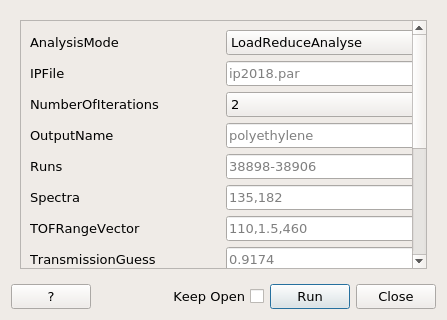
VesuvioAnalysis dialog.
Table of Contents
| Name | Direction | Type | Default | Description |
|---|---|---|---|---|
| AnalysisMode | Input | string | LoadReduceAnalyse | In the first case, all the algorithm is run. In the second case, the data are not re-loaded, and only the TOF and y-scaling bits are run. In the third case, only the y-scaling final analysis is run. In the fourth case, the data is re-loaded and the TOF bits are run. In the fifth case, only the TOF bits are run. Allowed values: [‘LoadReduceAnalyse’, ‘ReduceAnalyse’, ‘Analyse’, ‘LoadReduce’, ‘Reduce’] |
| IPFile | Input | string | Mandatory | The instrument parameter file. Allowed values: [‘par’] |
| NumberOfIterations | Input | number | 2 | Number of time the reduction is reiterated. Allowed values: [‘0’, ‘1’, ‘2’, ‘3’, ‘4’] |
| OutputName | Input | string | polyethylene | The base name for the outputs. |
| Runs | Input | string | 38898-38906 | List of Vesuvio run numbers (e.g. 20934-20937, 30924) |
| Spectra | Input | long list | 135,182 | Range of spectra to be analysed (first, last). Please note that spectra with a number lower than 135 are treated as back scattering spectra and are therefore not considered valid input as this algorithm is only for forward scattering data. |
| TOFRangeVector | Input | dbl list | 110,1.5,460 | In micro seconds (lower bound, binning, upper bound). |
| TransmissionGuess | Input | number | 0.9174 | A number from 0 to 1 to represent the experimental transmission value of the sample for epithermal neutrons. This value is used for the multiple scattering corrections. If 1, the multiple scattering correction is not run. |
| MultipleScatteringOrder | Input | number | 2 | Order of multiple scattering events in MC simultation. Allowed values: [‘1’, ‘2’, ‘3’, ‘4’] |
| MonteCarloEvents | Input | number | 1000000 | Number of events for MC multiple scattering simulation. |
| ComptonProfile | Input | TableWorkspace | Mandatory | Table for Compton profiles |
| ConstraintsProfile | Input | TableWorkspace | Table with LHS and RHS element of constraint on intensities of element peaks. A constraint can only be set when there are at least two elements in the ComptonProfile. For each constraint the ratio of the first to second intensities, each equal to atom stoichiometry times bound scattering cross section is defined in the column ScatteringCrossSection. Simple arithmetic can be included but the result may be rounded. The column State allows the values ‘eq’ and ‘ineq’. | |
| SpectraToBeMasked | Input | long list | ||
| SubtractResonancesFunction | Input | string | Function for resonance subtraction. Empty means no subtraction. | |
| YSpaceFitFunctionTies | Input | string | The TOF spectra are subtracted by all the fitted profiles about the first element specified in the elements string. Then such spectra are converted to the Y space of the first element (using the ConvertToYSPace algorithm). The spectra are summed together and symmetrised. A fit on the resulting spectrum is performed using a Gauss Hermite function up to the sixth order. |
This algorithm allows the loading, reduction, and analysis of forward scattering data obtained using Deep Inelastic Neutron Scattering (DINS), also referred to as Neutron Compton Scattering (NCS), at the VESUVIO spectrometer. The algorithm has been developed by the VESUVIO Instrument Scientists, Giovanni Romanelli and Matthew Krzystyniak. A previous version of the algorithm was described in: G. Romanelli et al.; Journal of Physics: Conf. Series 1055 (2018) 012016.
DINS allows the direct measurements of nuclear kinetic energies and momentum distributions, thus accessing the importance of nuclear quantum effects in condensed-matter systems, as well as the degree of anisotropy and anharmonicity in the local potentials affecting nuclei. DINS data appear as a collection of mass-resolved peaks (Neutron Compton Profiles, NCPs), that are fitted independently in the time-of-flight spectra, using the formalism of the Impulse Approximation and the y-scaling introduced by G. B. West.
Additional information about DINS theory and applications can be found in the recent review: C. Andreani et al., Advances in Physics, 66 (2017) 1-73
Additional information on the geometry and operations of the VESUVIO spectrometer can be found in J. Mayers and G. Reiter, Measurement Science and Technology, 23 (2012) 045902 G. Romanelli et al., Measurement Science and Technology, 28 (2017), 095501
Example: Analysis of polyethylene
# create table of elements
table = CreateEmptyTableWorkspace()
table.addColumn(type="str", name="Symbol")
table.addColumn(type="double", name="Mass (a.u.)")
table.addColumn(type="double", name="Intensity lower limit")
table.addColumn(type="double", name="Intensity value")
table.addColumn(type="double", name="Intensity upper limit")
table.addColumn(type="double", name="Width lower limit")
table.addColumn(type="double", name="Width value")
table.addColumn(type="double", name="Width upper limit")
table.addColumn(type="double", name="Centre lower limit")
table.addColumn(type="double", name="Centre value")
table.addColumn(type="double", name="Centre upper limit")
table.addRow(['H', 1.0079,  0.,1.,9.9e9,  3.,  4.5,  6.,  -1.5, 0., 0.5])
table.addRow(['C', 12.0,    0.,1.,9.9e9,  10., 15.5, 30., -1.5, 0., 0.5])

# create table of constraints
constraints = CreateEmptyTableWorkspace()
constraints.addColumn(type="int", name="LHS element")
constraints.addColumn(type="int", name="RHS element")
constraints.addColumn(type="str", name="ScatteringCrossSection")
constraints.addColumn(type="str", name="State")
constraints.addRow([0, 1, "2.*82.03/5.51", "eq"])

VesuvioAnalysis(IPFile = "ip2018.par", ComptonProfile = table, AnalysisMode = "LoadReduceAnalyse",
                NumberOfIterations = 2, OutputName = "polyethylene", Runs = "38898-38906", TOFRangeVector = [110.,1.5,460.],
                Spectra = [135,182], MonteCarloEvents = 1e3, ConstraintsProfile = constraints, SpectraToBeMasked = [173,174,181],
                SubtractResonancesFunction = 'name=Voigt,LorentzAmp=1.,LorentzPos=284.131,LorentzFWHM=2,GaussianFWHM=3;',
                YSpaceFitFunctionTies = "(c6=0., c4=0.)")

fit_results = mtd["polyethylene_H_JoY_sym_Parameters"]

print("variable", "value")
for row in range(fit_results.rowCount()):
    print(fit_results.column(0)[row],"{:.3f}".format(fit_results.column(1)[row]))
Output:
variable value
f1.sigma1 4.939
f1.c4 0.000
f1.c6 0.000
f1.A 0.080
f1.B0 0.000
Cost function value ...
Categories: AlgorithmIndex | Inelastic\Indirect\Vesuvio
Python: VesuvioAnalysis.py