\(\renewcommand\AA{\unicode{x212B}}\)

Stitch1D v3

Summary

Stitches single histogram matrix workspaces together

See Also

Rebin, Stitch1DMany

Properties

Name	Direction	Type	Default	Description
LHSWorkspace	Input	MatrixWorkspace	Mandatory	LHS input workspace.
RHSWorkspace	Input	MatrixWorkspace	Mandatory	RHS input workspace, must be same type as LHSWorkspace (histogram or point data).
OutputWorkspace	Output	MatrixWorkspace	Mandatory	Output stitched workspace.
StartOverlap	Input	number	Optional	Start overlap x-value in units of x-axis.
EndOverlap	Input	number	Optional	End overlap x-value in units of x-axis.
Params	Input	dbl list		Rebinning Parameters. See Rebin for format. If only a single value is provided, start and end are taken from input workspaces.
ScaleRHSWorkspace	Input	boolean	True	Scaling either with respect to LHS workspace or RHS workspace
UseManualScaleFactor	Input	boolean	False	True to use a provided value for the scale factor.
OutputScalingWorkspace	Input	string		Output WorkspaceSingleValue containing the scale factor and its error. No workspace creation if left empty.
ManualScaleFactor	Input	number	1	Provided value for the scale factor.
OutScaleFactor	Output	number		The actual used value for the scaling factor.

Description

Stitches single histogram Matrix Workspaces together outputting a stitched Matrix Workspace. The type of the input workspaces (histogram or point data) determines the stitch procedure. The x-error values Dx will always be ignored in case of histogram workspaces. Point data workspaces must be consistent, i.e. must have Dx defined or not.

Either the right-hand-side or left-hand-side workspace can be chosen to be scaled. Users can optionally provide Rebin v1 Params, otherwise they are calculated from the input workspaces. Likewise, StartOverlap and EndOverlap are optional. If not provided, then these are taken to be the region of X-axis intersection.

The algorithm workflow for histograms is as follows:

1. The workspaces are initially rebinned, as prescribed by the rebin Params. Note that rebin parameters are determined automatically if not provided. In this case, the step size is taken from the step size of the LHS workspace (or from the RHS workspace if ScaleRHSWorkspace was set to false) and rebin boundaries are taken from the minimum X value in the LHS workspace and the maximum X value in the RHS workspace respectively.

2. After rebinning, each spectrum is searched for special values. Special values refer to signal (Y) and error (E) values that are either infinite or NaN. These special values are masked out as zeroes and their positions are recorded for later reinsertion.

3. Next, if UseManualScaleFactor was set to false, both workspaces will be integrated according to the integration range defined by StartOverlap and EndOverlap. Note that the integration is performed without special values, as those have been masked out in the previous step. The scale factor is then calculated as the quotient of the integral of the left-hand-side workspace by the integral of the right-hand-side workspace (or the quotient of the right-hand-side workspace by the left-hand-side workspace if ScaleRHSWorkspace was set to false), and the right-hand-side workspace (left-hand-side if ScaleRHSWorkspace was set to false) is multiplied by the calculated factor.

4. Alternatively, if UseManualScaleFactor was set to true, the scale factor is applied to the right-hand-side workspace (left-hand-side workspace if ScaleRHSWorkspace was set to false).

5. The weighted mean of the two workspaces in range [StartOverlap, EndOverlap] is calculated. Note that if both workspaces have zero errors, an un-weighted mean will be performed instead.

6. The output workspace will be created by summing the left-hand-side workspace (values in range [StartX, StartOverlap], where StartX is the minimum X value specified via Params or calculated from the left-hand-side workspace) + weighted mean workspace + right-hand-side workspace (values in range [EndOverlap, EndX], where EndX is the maximum X value specified via Params or calculated from the right-hand-side workspace) multiplied by the scale factor. Dx values will not be present in the output workspace.

7. The special values are put back in the output workspace. Note that if both the left-hand-side workspace and the right-hand-side workspace happen to have a different special value in the same bin, this bin will be set to infinite in the output workspace.

Below is a flowchart illustrating the steps in the algorithm (it assumes ScaleRHSWorkspace is true). Figure on the left corresponds to the workflow when no scale factor is provided, while figure on the right corresponds to workflow with a manual scale factor specified by the user.

The algorithm workflow for point data is as follows:

1. If UseManualScaleFactor was set to false, both workspaces will be integrated according to the integration range defined by StartOverlap and EndOverlap. Note that the integration is performed without special values, as those have been masked out in the previous step. The scale factor is then calculated as the quotient of the integral of the left-hand-side workspace by the integral of the right-hand-side workspace (or the quotient of the right-hand-side workspace by the left-hand-side workspace if ScaleRHSWorkspace was set to false), and the right-hand-side workspace (left-hand-side if ScaleRHSWorkspace was set to false) is multiplied by the calculated factor.

2. Alternatively, if UseManualScaleFactor was set to true, the scale factor is applied to the right-hand-side workspace (left-hand-side workspace if ScaleRHSWorkspace was set to false).

3. The output workspace will be created by joining using ConjoinXRuns v1 and sorting using SortXAxis v1. Dx values will be present in the output workspace.

Error propagation

Errors are are handled and propagated in every step according to Error Propagation. This includes every child algorithm: Rebin v1, Integration v1, Divide v1, Multiply v1 and WeightedMean v1. In particular, when the scale factor is calculated as the quotient of the left-hand-side integral and the right-hand-side integral, the result is a number with an error associated, and therefore the multiplication of the right-hand-side workspace by this number takes into account its error.

Usage

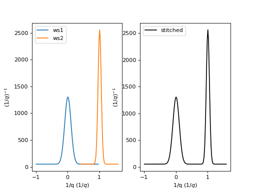
Example - a basic example using stitch1D to stitch two histogram workspaces together.

from mantid.simpleapi import *
import matplotlib.pyplot as plt
import numpy as np

def gaussian(x, mu, sigma):
  """Creates a Gaussian peak centered on mu and with width sigma."""
  return (1/ sigma * np.sqrt(2 * np.pi)) * np.exp( - (x-mu)**2  / (2*sigma**2))

# create two histograms with a single peak in each one
x1 = np.arange(-1, 1, 0.02)
x2 = np.arange(0.4, 1.6, 0.02)
ws1 = CreateWorkspace(UnitX="1/q", DataX=x1, DataY=gaussian(x1[:-1], 0, 0.1)+1)
ws2 = CreateWorkspace(UnitX="1/q", DataX=x2, DataY=gaussian(x2[:-1], 1, 0.05)+1)

# stitch the histograms together
stitched, scale = Stitch1D(LHSWorkspace=ws1, RHSWorkspace=ws2, StartOverlap=0.4, EndOverlap=0.6, Params=0.02)

# plot the individual workspaces alongside the stitched one
fig, axs = plt.subplots(nrows=1, ncols=2, subplot_kw={'projection':'mantid'})

axs[0].plot(mtd['ws1'], wkspIndex=0, label='ws1')
axs[0].plot(mtd['ws2'], wkspIndex=0, label='ws2')
axs[0].legend()
axs[1].plot(mtd['stitched'], wkspIndex=0, color='k', label='stitched')
axs[1].legend()

# uncomment the following line to show the plot window
#fig.show()

(Source code, png, hires.png, pdf)

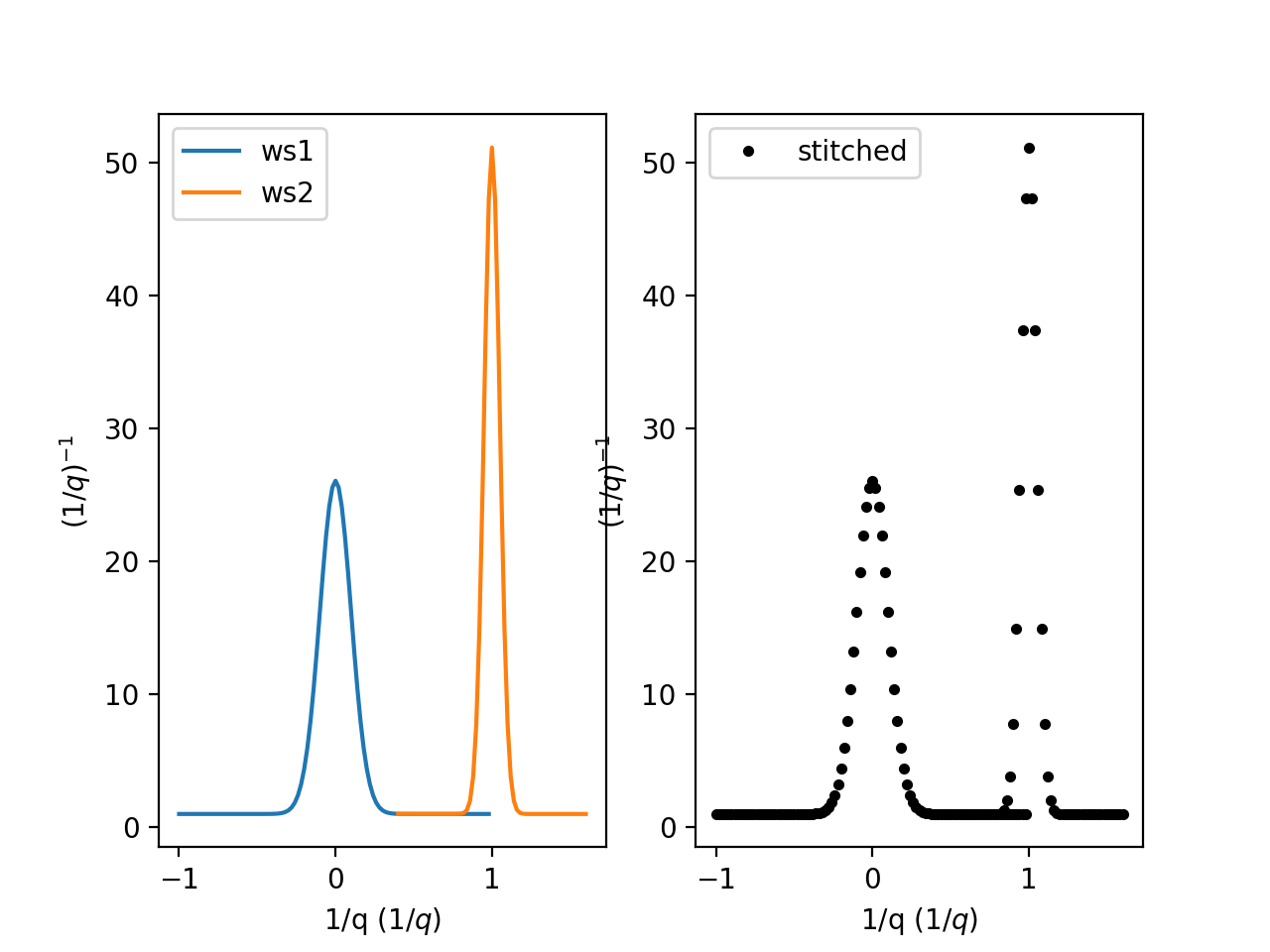
Example - a basic example using stitch1D to stitch two point data workspaces together.

from mantid.simpleapi import *
import matplotlib.pyplot as plt
import numpy as np

def gaussian(x, mu, sigma):
  """Creates a Gaussian peak centered on mu and with width sigma."""
  return (1/ sigma * np.sqrt(2 * np.pi)) * np.exp( - (x-mu)**2  / (2*sigma**2))

# create two histograms with a single peak in each one
x1 = np.arange(-1, 1, 0.02)
x2 = np.arange(0.4, 1.6, 0.02)
ws1 = CreateWorkspace(UnitX="1/q", DataX=x1, DataY=gaussian(x1, 0, 0.1)+1)
ws2 = CreateWorkspace(UnitX="1/q", DataX=x2, DataY=gaussian(x2, 1, 0.05)+1)

# stitch the histograms together
stitched, scale = Stitch1D(LHSWorkspace=ws1, RHSWorkspace=ws2, StartOverlap=0.4, EndOverlap=0.6)

# plot the individual workspaces alongside the stitched one
fig, axs = plt.subplots(nrows=1, ncols=2, subplot_kw={'projection':'mantid'})

axs[0].plot(mtd['ws1'], wkspIndex=0, label='ws1')
axs[0].plot(mtd['ws2'], wkspIndex=0, label='ws2')
axs[0].legend()
axs[1].plot(mtd['stitched'], wkspIndex=0, color='k', marker='.', ls='', label='stitched')
axs[1].legend()

# uncomment the following line to show the plot window
#fig.show()

(Source code, png, hires.png, pdf)

Example - a practical example using reflectometry data and a scale factor.

from mantid.simpleapi import *
import matplotlib.pyplot as plt

try:
   trans1 = Load('INTER00013463')
   trans2 = Load('INTER00013464')

   trans1_wav = CreateTransmissionWorkspaceAuto(trans1)
   trans2_wav = CreateTransmissionWorkspaceAuto(trans2)

   stitched_wav, y = Stitch1D(trans1_wav, trans2_wav, UseManualScaleFactor=True, ManualScaleFactor=0.85)

   # plot the individual and stitched workspaces next to each other
   fig, axs = plt.subplots(nrows=1, ncols=2, subplot_kw={'projection':'mantid'})

   axs[0].plot(trans1_wav, wkspIndex=0, label=str(trans1_wav))
   axs[0].plot(trans2_wav, wkspIndex=0, label=str(trans2_wav))
   axs[0].legend()
   # use same y scale on both plots
   ylimits = axs[0].get_ylim()
   axs[1].plot(stitched_wav, wkspIndex=0, color='k', label='stitched')
   axs[1].legend()
   axs[1].set_ylim(ylimits)

   # uncomment the following line to show the plot window
   #fig.show()
except ValueError:
   print("Cannot load data")

(Source code, png, hires.png, pdf)

Categories: AlgorithmIndex | Reflectometry

Source

C++ header: Stitch1D.h

C++ source: Stitch1D.cpp