\(\renewcommand\AA{\unicode{x212B}}\)

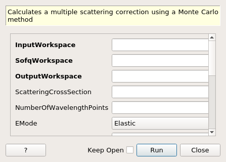
DiscusMultipleScatteringCorrection v1¶

DiscusMultipleScatteringCorrection dialog.

Table of Contents

Summary
- See Also
Properties
Description
Usage
Source

Summary ¶

Calculates a multiple scattering correction using a Monte Carlo method

Properties ¶

Name	Direction	Type	Default	Description
InputWorkspace	Input	MatrixWorkspace	Mandatory	The name of the input workspace. The input workspace must have X units of wavelength. This is used to supply the detector positions and the x axis range to calculate corrections for
SofqWorkspace	Input	MatrixWorkspace	Mandatory	The name of the workspace containing S’(q). The input workspace must contain a single spectrum and have X units of momentum transfer.
OutputWorkspace	Output	WorkspaceGroup	Mandatory	Name for the WorkspaceGroup that will be created. Each workspace in the group contains a calculated weight for a particular number of scattering events. The number of scattering events varies from 1 up to the number supplied in the NumberOfScatterings parameter. The group will also include an additional workspace for a calculation with a single scattering event where the absorption post scattering has been set to zero
ScatteringCrossSection	Input	MatrixWorkspace		A workspace containing the scattering cross section as a function of k, \(\sigma_s(k)\)
NumberOfWavelengthPoints	Input	number	Optional	The number of wavelength points for which a simulation is attempted if ResimulateTracksForDifferentWavelengths=true
EMode	Input	string	Elastic	The energy mode (default: Elastic). Allowed values: [‘Elastic’, ‘Direct’, ‘Indirect’]
NeutronPathsSingle	Input	number	1000	The number of “neutron” paths to generate for single scattering
NeutronPathsMultiple	Input	number	1000	The number of “neutron” paths to generate for multiple scattering
SeedValue	Input	number	123456789	Seed the random number generator with this value
NumberScatterings	Input	number	2	Number of scatterings
Interpolation	Input	string	Linear	Method of interpolation used to compute unsimulated values. Allowed values: [‘Linear’, ‘CSpline’]
SparseInstrument	Input	boolean	False	Enable simulation on special instrument with a sparse grid of detectors interpolating the results to the real instrument.
NumberOfDetectorRows	Input	number	5	Number of detector rows in the detector grid of the sparse instrument.
NumberOfDetectorColumns	Input	number	10	Number of detector columns in the detector grid of the sparse instrument.
ImportanceSampling	Input	boolean	False	Enable importance sampling on the Q value chosen on multiple scatters based on Q.S(Q)
MaxScatterPtAttempts	Input	number	5000	Maximum number of tries made to generate a scattering point within the sample. Objects with holes in them, e.g. a thin annulus can cause problems if this number is too low. If a scattering point cannot be generated by increasing this value then there is most likely a problem with the sample geometry.

This algorithm calculates a Multiple Scattering correction using a Monte Carlo integration method. The method uses a structure function for the sample to determine the probability of a particular q value for each scattering event and it doesn’t therefore rely on an assumption that the scattering is isotropic.

The structure function that the algorithm takes as input is a linear combination of the coherent and incoherent structure factors:

\(S'(Q) = \frac{1}{\sigma_b}(\sigma_{coh} S(Q) + \sigma_{inc} S_s(Q))\)

If the sample is a perfectly coherent scatterer then \(S'(Q) = S(Q)\)

The algorithm is based on code which was originally written in Fortran as part of the Discus program [1]. The code was subsequently resurrected and improved by Spencer Howells under the Muscat name and was included in the QENS MODES package [2] These original programs calculated multiple scattering corrections for inelastic instruments but an elastic diffraction version of the code was also created and results from that program are included in this paper by Mancinelli [3].

This algorithm so far only considers the elastic case but the intention is to extend this to include inelastic at a later date following the approach in the Discus\MODES programs.

Theory ¶

The algorithm calculates a set of dimensionless weights \(J_n\) describing the probability of detection at an angle \(\theta\) after n scattering events given a total incident flux \(I_0\) and a transmitted flux of T:

\(T_n(\theta,\lambda) = J_n I_0(\lambda)\)

The quantity \(J_n\) is calculated by performing the following integration:

\[\begin{split}J_n &= (\frac{\mu_s}{4 \pi})^n \frac{1}{A} \int dS \int_{0}^{l_1^{max}} dl_1 e^{-\mu_T l_1} \prod\limits_{i=1}^{n-1} [\int_{0}^{l_{i+1}^{max}} dl_{i+1} \int_{0}^{\pi} \sin\theta_i d\theta_i \int_{0}^{2 \pi} d\phi_i (e^{-\mu_T l_{i+1}}) S(Q_i)] e^{-\mu_T l_{out}} S(Q_n) \\ &=(\frac{\mu_s}{4 \pi})^n \frac{1}{A} \int dS \int_{0}^{l_1^{max}} dl_1 e^{-\mu_T l_1} \prod\limits_{i=1}^{n-1} [\int_{0}^{l_{i+1}^{max}} dl_{i+1} \int_{0}^{2k} dQ_i \int_{0}^{2 \pi} d\phi_i (e^{-\mu_T l_{i+1}}) \frac{Q_i}{k^2} S(Q_i)] e^{-\mu_T l_{out}} S(Q_n)\end{split}\]

The variables \(l_i^{max}\) represent the maximum path length before the next scatter given a particular phi and theta value (Q). Each \(l_i\) is actually a function of all of the earlier values for the \(l_i\), \(\phi\) and \(Q\) variables ie \(l_i = l_i(l_1, l_2, ..., l_{i-1}, \phi_1, \phi_2, ..., \phi_i, Q_1, Q_2, ..., Q_i)\)

The following substitutions are then performed in order to make it more convenient to evaluate as a Monte Carlo integral:

\(t_i = \frac{1-e^{-\mu_T l_i}}{1-e^{-\mu_T l_i^{max}}}\)

\(u_i = \frac{\phi_i}{2 \pi}\)

\(2 k^2 = \frac{\sigma_S \int_0^{2k} Q_i S(Q_i) dQ}{\sigma_s(k)}\)

Using the new variables the integral is:

\[J_n = \frac{1}{A} \int dS \int_{0}^{1} dt_1 \frac{1-e^{-\mu_T l_1^{\ max}}}{\sigma_T} \prod\limits_{i=1}^{n-1}[\int_{0}^{1} dt_{i+1} \int_{0}^{2k} dQ_i \int_{0}^{1} du_i \frac{(1-e^{-\mu_T l_{i+1}^{max}})}{\sigma_T} \frac{Q_i}{\int_0^{2k} Q_i S(Q_i) dQ_i} S(Q_i) \sigma_s(k)] e^{-\mu_T l_{out}} S(Q_n) \frac{\sigma_s}{4 \pi}\]

This is evaluated as a Monte Carlo integration by selecting random values for the variables \(t_i\) and \(u_i\) between 0 and 1 and values for \(Q_i\) between 0 and 2k. A simulated path is traced through the sample to enable the \(l_i^{\ max}\) values to be calculated. The path is traced by calculating the \(l_i\), \(\theta\) and \(\phi\) values as follows from the random variables. The code keeps a note of the start coordinates of the current path segment and updates it when moving to the next segment using these randomly selected lengths and directions:

\(l_i = -\frac{1}{\mu_T}ln(1-(1-e^{-\mu_T l_i^{\ max}})t_i)\)

\(\cos\theta_i = 1 - Q_i^2/k^2\)

\(\phi_i = 2 \pi u_i\)

The final Monte Carlo integration that is actually performed by the code is as follows where N is the number of scenarios:

\[J_n = \frac{1}{N}\sum \frac{1-e^{-\mu_T l_1^{\ max}}}{\sigma_T} \prod\limits_{i=1}^{n-1}[\frac{(1-e^{-\mu_T l_{i+1}^{max}})}{\sigma_T} \frac{Q_i}{<Q S(Q)>} S(Q_i) \sigma_s(k)] e^{-\mu_T l_{out}} S(Q_n) \frac{\sigma_s}{4 \pi}\]

The purpose of replacing \(2 k^2\) with \(\int Q S(Q) dQ\) can now be seen because it avoids the need to multiply by an integration range across \(dQ\) when converting the integral to a Monte Carlo integration. This is useful in the inelastic version of this algorithm where the integration of the structure factor is over two dimensions \(Q\) and \(\omega\) and the area of \(Q\omega\) space that has been integrated over is less obvious.

This is similar to the formulation described in the Mancinelli paper except there is no random variable to decide whether a particular scattering event is coherent or incoherent.

Importance Sampling ¶

The algorithm includes an option to use importance sampling to improve the results for S(Q) profiles containing spikes. Without this option enabled, the contribution from rare, high values in the structure factor is only visible at a very high number of scenarios.

The importance sampling is achieved using a further change of variables as follows:

\(v_i = P(Q_i) = \frac{I(Q_i)}{I(2k)}\) where \(I(x) = \int_{0}^{x} Q S(Q) dQ\)

With this approach the Q value for each segment is chosen as follows based on a \(v_i\) value randomly selected between 0 and 1:

\(Q_i = P^{-1}(v_i)\)

\(\cos\theta_i\) is determined from \(Q_i\) as before. The change of variables gives the following integral for \(J_n\):

\[ \begin{align}\begin{aligned}J_n = \frac{1}{A} \int dS \int_{0}^{1} dt_1 \frac{1-e^{-\mu_T l_1^{\ max}}}{\sigma_T} \prod\limits_{i=1}^{n-1}[\int_{0}^{1} dt_{i+1} \int_{0}^{1} dv_i 2 \frac{I(2k)}{2k^2} \sigma_s \int_{0}^{1} du_i \frac{(1-e^{-\mu_T l_{i+1}^{max}})}{\sigma_T}] e^{-\mu_T l_{out}} S(Q_n) \frac{\sigma_s}{4 \pi}\\J_n = \frac{1}{A} \int dS \int_{0}^{1} dt_1 \frac{1-e^{-\mu_T l_1^{\ max}}}{\sigma_T} \prod\limits_{i=1}^{n-1}[\int_{0}^{1} dt_{i+1} \int_{0}^{1} dv_i 2 \sigma_s(k) \int_{0}^{1} du_i \frac{(1-e^{-\mu_T l_{i+1}^{max}})}{\sigma_T}] e^{-\mu_T l_{out}} S(Q_n) \frac{\sigma_s}{4 \pi}\end{aligned}\end{align} \]

Finally, the equivalent Monte Carlo integration that the algorithm performs with importance sampling enabled is:

\[J_n = \frac{1}{N}\sum \frac{1-e^{-\mu_T l_1^{\ max}}}{\sigma_T} \prod\limits_{i=1}^{n-1}[2 \sigma_s(k) \frac{(1-e^{-\mu_T l_{i+1}^{max}})}{\sigma_T}] e^{-\mu_T l_{out}} S(Q_n) \frac{\sigma_s}{4 \pi}\]

Outputs ¶

The algorithm outputs a workspace group containing the following workspaces:

Several workspaces called Scatter_n where n is the number of scattering events considered. Each workspace contains “per detector” weights as a function of wavelength for a specific number of scattering events. The number of scattering events ranges between 1 and the number specified in the NumberOfScatterings parameter
A workspace called Scatter_1_NoAbsorb is also created for a scenario where neutrons are scattered once, absorption is assumed to be zero and re-scattering after the simulated scattering event is assumed to be zero. This is the quantity \(J_{1}^{*}\) described in the Discus manual
A workspace called Scatter_2_n_Summed which is the sum of the Scatter_n workspaces for n > 1

The output can be applied to a workspace containing a real sample measurement in one of two ways:

subtraction method. The additional intensity contributed by multiple scattering to either a raw measurement or a vanadium corrected measurement can be calculated from the weights output from this algorithm. The additional intensity can then be subtracted to give an idealised “single scatter” intensity. For example, the additional intensity measured at a detector due to multiple scattering is given by \((\sum_{n=2}^{\infty} J_n) E(\lambda) I_0(\lambda) \Delta \Omega\) where \(E(\lambda)\) is the detector efficiency, \(I_0(\lambda)\) is the incident intensity and \(\Delta \Omega\) is the solid angle subtended by the detector. The factors \(E(\lambda) I_0(\lambda) \Delta \Omega\) can be obtained from a Vanadium run - although to take advantage of the “per detector” multiple scattering weights, the preparation of the Vanadium data will need to take place “per detector” instead of on focussed datasets
factor method. The correction can be applied by multiplying the real sample measurement by \(J_1/\sum_{n=1}^{\infty} J_n\). This approach avoids having to create a suitably normalised intensity from the weights and the method is also more tolerant of any normalisation inaccuracies in the S(Q) profile

The multiple scattering correction should be applied before applying an absorption correction.

The Discus manual describes a further method of applying an attenuation correction and a multiple scattering correction in one step using a variation of the factor method. To achieve this the real sample measurement should be multipled by \(J_1^{*}/(\sum_{n=1}^{\infty} J_n\)). Note that this differs from the approach taken in other Mantid absorption correction algorithms such as MonteCarloAbsorption because of the properties of \(J_{1}^{*}\). \(J_{1}^{*}\) corrects for attenuation due to absorption before and after the simulated scattering event (which is the same as MonteCarloAbsorption) but it only corrects for attenuation due to scattering after the simulated scattering event. For this reason it’s not clear this feature from Discus is useful but it has been left in for historical reasons.

The sample shape can be specified by running the algorithms SetSample or LoadSampleShape on the input workspace prior to running this algorithm.

The algorithm can take a long time to run on instruments with a lot of spectra andor a lot of bins in each spectrum. The run time can be reduced by enabling the following interpolation features:

the multiple scattering correction can be calculated on a subset of the wavelength bins in the input workspace by specifying a non-default value for NumberOfWavelengthPoints. The other wavelength points will be calculated by interpolation
the algorithm can be performed on a subset of the detectors by setting SparseInstrument=True

Both of these interpolation features are described further in the documentation for the MonteCarloAbsorption algorithm

References ¶

[1]	M W Johnson, 1974 AERE Report R7682, Discus: A computer program for the calculating of multiple scattering effects in inelastic neutron scattering experiments

[2]	WS Howells, V Garcia Sakai, F Demmel, MTF Telling, F Fernandez-Alonso, Feb 2010, MODES manual RAL-TR-2010-006, doi: 10.5286/raltr.2010006

[3]	R Mancinelli 2012 J. Phys.: Conf. Ser. 340 012033, Multiple neutron scattering corrections. Some general equations to do fast evaluations doi: 10.1088/1742-6596/340/1/012033