\(\renewcommand\AA{\unicode{x212B}}\)
Contents
The documentation on this wiki page is the full detailed description of the syntax you can use in an IDF to describe an instrument (note parameters of instrument components may optionally be stored in parameter file).
To get started creating an IDF follow the instructions on the Create an IDF page, then return here for more detailed explanations of syntax and structures.
An instrument definition file (IDF) aims to describe an instrument, in particular providing details about those components of the instruments that are critically affecting the observed signal from an experiment. Parameter values of components may also be specified such as information about the opening height of a slit, the final energy of a detector and so on. The value of such parameters can optionally be linked to values stored in log-files.
In summary an IDF may be used to describe any or all of the following:
An IDF is structured as an XML document. For the purpose here it is enough to know that an XML document follows a tree-based structure of elements with attributes. For example:
<type name="main-detector-bank">
  <component type="main-detector-pixel" >
    <location x="-0.31" y="0.1" z="0.0" />
    <location x="-0.32" y="0.1" z="0.0" />
    <location x="-0.33" y="0.1" z="0.0" />
  </component>
</type>
defines an XML element with has the attribute name=”main-detector-bank”. This element contains one sub-element , which again contains 3 elements. In plain English the above XML code aims to describe a “main-detector-bank” that contains 3 detector pixels and their locations within the bank.
If a component is a cylindrical tube where slices of this types are treated as detector pixels the tube detector performance enhancement can optionally be used, which will e.g. make the display of this tube in the instrument viewer faster. This can be done by adding ‘outline’ attribute to the tag and setting its value to “yes”.
<type name="standard-tube" outline="yes">
  <component type="standard-pixel" >
    <location y="-1.4635693359375"/>
    <location y="-1.4607080078125"/>
    <location y="-1.4578466796875"/>
  </component>
</type>
The ‘outline attribute’ only affects the 3D view of the instrument, which appears by default. It may lead to a less accurate placing of the detector pixels and in particular may not show the effects of tube calibration. However a 2D view of the instrument will still place pixel detectors accurately.
An IDF can be loaded manually from any file with extension .xml or .XML using LoadInstrument or LoadEmptyInstrument.
When loading a data file if the file has an embedded mantid instrument definition (as in some nexus files) then this one will be used, otherwise we will attempt to determine a matching file from the IDFs located in the MantidInstall instrument directory.
To be found automatically Instrument definition files are required to have the format INSTRUMENTNAME_DefinitionANYTHING.xml, where INSTRUMENTNAME is the name of the instrument and ANYTHING can be any string including an empty string. Where more than one IDF is defined for an instrument the appropriate IDF is loaded based on its valid-from date. Note for this to work the Workspace for which an IDF is loaded into must contain a record of when the data were collected. This information is taken from the workspace’s Run object, more specifically the run_start property of this object.
You can determine which file would be selected for an instrument and date using the following python:
Example: Getting the right instrument filename
# if no date is given it will default to returning the IDF filename that is currently valid.
from mantid.api import ExperimentInfo
currentIDF = ExperimentInfo.getInstrumentFilename("ARCS")
otherIDF = ExperimentInfo.getInstrumentFilename("ARCS", "2012-10-30T00:00:00")
Mantid ships with many instrument definition files within the installation but also has the capability of fetching new instrument definitions by running the DownloadInstrument algorithm (this is run automatically on startup). Downloaded definitions are written to a different directory to the shipped versions so that they do not overwrite them. The default list of directories searched (in the this order) for an IDF for a given instrument are:
For Windows:
For Linux/OSX:
You should not edit files in the downloaded location, or add new ones as the may be deleted or overwritten. If you have a change to an instrument definition you wish to use then edit a copy in the [INSTALLDIR] instrument directory, but update the valid-from date so mantid will pick that one up in preference. Or if you just wish to force a particular instrument definition for a particular workspace just run LoadInstrument for that workspace.
For information on how to define geometric shapes see HowToDefineGeometricShape.
<instrument> is the top level XML element of an IDF. It takes attributes, three of which must be included. An example is
<instrument xmlns="http://www.mantidproject.org/IDF/1.0"
            xmlns:xsi="http://www.w3.org/2001/XMLSchema-instance"
            xsi:schemaLocation="http://www.mantidproject.org/IDF/1.0 http://schema.mantidproject.org/IDF/1.0/IDFSchema.xsd"
            name="ARCS"
            valid-from="1900-01-31 23:59:59"
            valid-to="2100-01-31 23:59:59">
Of the attributes in the example above
(+) Both valid-from and valid-to are required to be set using the ISO 8601 date-time format, i.e. as YYYY-MM-DD HH:MM:SS or YYYY-MM-DDTHH:MM:SS 2. Valid ranges may overlap, provided the valid-from times are all different. If several files are currently valid, the one with the most recent valid-from time is selected.
Use the element to define a physical part of the instrument. A requires two things
Here is an example
<component type="slit" name="bob">
  <location x="10.651"/>
  <location x="11.983"/>
</component>

<type name="slit"></type>
Which defined two slits at two difference locations. Optionally a <component> can be given a ‘name’, in the above example this name is “bob”. If no ‘name’ attribute is specified the name of the <component> defaults to the ‘type’ string, in the above this is “slit”. Giving sensible names to components is recommended for a number of reasons including #. The ‘Instrument Tree’ view of an instrument viewer uses these names #. when specifying <parameter>s through <component-link>s these names are used.
Within Mantid certain <type>s have special meaning. A special <type> is specified by including an ‘is’ attribute as demonstrated below
<type name="pixel" is="detector">
  <cuboid id="app-shape">
    <left-front-bottom-point x="0.0025" y="-0.1" z="0.0"  />
    <left-front-top-point  x="0.0025" y="-0.1" z="0.0002"  />
    <left-back-bottom-point  x="-0.0025" y="-0.1" z="0.0"  />
    <right-front-bottom-point  x="0.0025" y="0.1" z="0.0"  />
  </cuboid>
</type>
where the ‘is’ attribute of is used to say this is a detector-<type> (note this particular detector-<type> has been assigned a geometric shape, in this case a cuboid, see HowToDefineGeometricShape). Special types recognised are:
For example it is important to specify the location of one Source-<type> and one SamplePos-<type> in order for Mantid to be able to calculate L1 and L2 distances and convert time-of-flight to, for instance, d-spacing. An example of specifying a Source and SamplePos is shown below
<component type="neutron moderator"> <location z="-10.0"/> </component>
<type name="neutron moderator" is="Source"/>

<component type="some sample holder"> <location /> </component>
<type name="some sample holder" is="SamplePos" />
Any component that is either a detector or monitor must be assigned a unique detector/monitor ID numbers (note this is not spectrum numbers but detector/monitor ID numbers). There are at least two important reason to insist on this.
Warning
As of version 3.12 of Mantid, Instruments in Mantid will no longer silently discard detectors defined with duplicate IDs. Detector IDs (including Monitors) must be unique across the Instrument. IDFs cannot be loaded if they violate this.
The <idlist> element and the idlist attribute of the elements is used to assign detector IDs. The notation for using idlist is
<component type="monitor" idlist="monitor-id-list">
  <location r="5.15800" t="180.0" p="0.0" /> <!-- set to ID=500 in list below -->
  <location r="5.20400" t="180.0" p="0.0" /> <!-- set to ID=510 -->
  <location r="5.30400" t="180.0" p="0.0" /> <!-- set to ID=520 -->
  <location r="5.40400" t="180.0" p="0.0" /> <!-- set to ID=531 -->
  <location r="6.10400" t="180.0" p="0.0" /> <!-- set to ID=611 -->
  <location r="6.24700" t="0.000" p="0.0" /> <!-- set to ID=612 -->
  <location r="6.34700" t="0.000" p="0.0" /> <!-- set to ID=613 -->
  <location r="6.50000" t="0.000" p="0.0" /> <!-- set to ID=650 -->
</component>

<type name="monitor" is="monitor"/>

<idlist idname="monitor-id-list">
  <id start="500" step="10" end="530" />  <!-- specifies IDs: 500, 510, 520, 530 -->
  <id start="611" end="613" />            <!-- specifies IDs: 611, 612 and 613 -->
  <id val="650" />                        <!-- specifies ID: 650 -->
</idlist>
As can be seen to specify a sequence of IDs use the notation <id start=”500” step=”10” end=”530” />, where if the step attribute defaults to step=”1” if it is left out. Just specify just a single ID number you may alternatively use the notation <id val=”650” />. Please note the number of ID specified must match the number of detectors/monitors defined.
There is a shortcut way to create 3D arrays of detector pixels. These pixels represent volumetric detectors. Here is an example how to do this:
<component type="block"  idstart="1" idfillorder="zxy">
  <location x="0" y="0" z="0.2" name="bank2">
  </location>
</component>

<type name="block" is="GridDetector" type="voxel"
    xpixels="4" xstart="-0.04" xstep="+0.02"
    ypixels="48" ystart="-0.48" ystep="+0.02"
    zpixels="16" zstart="-0.08" zstep="+0.01">
  <properties/>
</type>

<!-- Pixel for Detectors-->
<type name="voxel" is="detector">
    <cuboid id="shape">
            <left-front-bottom-point x="-0.01" y="-0.01" z="-0.005"  />
            <left-front-top-point  x="-0.01" y="0.01" z="-0.005"  />
            <left-back-bottom-point  x="0.01" y="-0.01" z="-0.005"  />
            <right-front-bottom-point  x="-0.01" y="-0.01" z="0.005"  />
    </cuboid>
<algebra val="shape" />
</type>
There is a shortcut way to create 2D arrays of detector pixels. Here is an example of how to do it:
<component type="panel"  idstart="1000" idfillbyfirst="y" idstepbyrow="300">
  <location r="0" t="0" name="bank1">
  </location>
</component>

<component type="panel"  idstart="100000" idfillbyfirst="y" idstepbyrow="300">
  <location r="45.0" t="0" name="bank2">
  </location>
</component>

<!-- Rectangular Detector Panel. Position 100 "pixel" along x from -0.1 to 0.1
     and 200 "pixel" along y from -0.2 to 0.2 (relative to the coordinate system of the bank) -->
<type name="panel" is="RectangularDetector" type="pixel"
    xpixels="100" xstart="-0.100" xstep="+0.002"
    ypixels="200" ystart="-0.200" ystep="+0.002" >
</type>

<!-- Pixel for Detectors. Shape defined to be a (0.001m)^2 square in XY-plane with tickness 0.0001m -->
<type is="detector" name="pixel">
  <cuboid id="pixel-shape">
    <left-front-bottom-point y="-0.001" x="-0.001" z="0.0"/>
    <left-front-top-point y="0.001" x="-0.001" z="0.0"/>
    <left-back-bottom-point y="-0.001" x="-0.001" z="-0.0001"/>
    <right-front-bottom-point y="-0.001" x="0.001" z="0.0"/>
  </cuboid>
  <algebra val="pixel-shape"/>
</type>
In the previous example, we saw that Rectangular Detectors provide a simple way of producing detectors with regular topology and geometry. The StructuredDetector provides a way of producing detectors with regular topology and irregular geometry. It can be thought of as a warped RectangularDetector:
<component name="DetectorBank" type="fan" idstart="0" idfillfirst="y" idstepbyrow="100" idstep="1">
  <location />
</component>

<type name="fan" is="StructuredDetector" xpixels="4" ypixels="5" type="pixel">
   <vertex x="-0.0" y="0.0" z="0.0" />
   <vertex x="-0.0" y="0.0" z="0.0" />
   <vertex x="0.0" y="0.0" z="0.0" />
   <vertex x="0.0" y="0.0" z="0.0" />
   <vertex x="0.0" y="0.0" z="0.0" />
   <vertex x="-0.00138071187457" y="0.00333333333333" z="0.0" />
   <vertex x="-0.000663041224598" y="0.00333333333333" z="0.0" />
   <vertex x="0.0" y="0.00333333333333" z="0.0" />
   <vertex x="0.000663041224597" y="0.00333333333333" z="0.0" />
   <vertex x="0.00138071187457" y="0.00333333333333" z="0.0" />
   <vertex x="-0.00276142374915" y="0.00666666666667" z="0.0" />
   <vertex x="-0.0013260824492" y="0.00666666666667" z="0.0" />
   <vertex x="0.0" y="0.00666666666667" z="0.0" />
   <vertex x="0.00132608244919" y="0.00666666666667" z="0.0" />
   <vertex x="0.00276142374915" y="0.00666666666667" z="0.0" />
   <vertex x="-0.00414213562372" y="0.01" z="0.0" />
   <vertex x="-0.00198912367379" y="0.01" z="0.0" />
   <vertex x="0.0" y="0.01" z="0.0" />
   <vertex x="0.00198912367379" y="0.01" z="0.0" />
   <vertex x="0.00414213562372" y="0.01" z="0.0" />
   <vertex x="-0.0055228474983" y="0.0133333333333" z="0.0" />
   <vertex x="-0.00265216489839" y="0.0133333333333" z="0.0" />
   <vertex x="0.0" y="0.0133333333333" z="0.0" />
   <vertex x="0.00265216489839" y="0.0133333333333" z="0.0" />
   <vertex x="0.00552284749829" y="0.0133333333333" z="0.0" />
   <vertex x="-0.00690355937287" y="0.0166666666667" z="0.0" />
   <vertex x="-0.00331520612299" y="0.0166666666667" z="0.0" />
   <vertex x="0.0" y="0.0166666666667" z="0.0" />
   <vertex x="0.00331520612299" y="0.0166666666667" z="0.0" />
   <vertex x="0.00690355937287" y="0.0166666666667" z="0.0" />
</type>

<type is="detector" name="pixel"/>
The <location> element allows the specification of both the position of a component and a rotation or the component’s coordinate system. The position part can be specified either using standard x, y and z coordinates or using spherical coordinates: r, t and p, which stands for radius, theta and phi, t is the angle from the z-axis towards the x-axis and p is the azimuth angle in the xy-plane 3. Examples of translations include
<component type="something" name="bob">
  <location x="1.0" y="0.0" z="0.0" name="benny" />
  <location r="1.0" t="90.0" p="0.0"/>
</component>
The above two translations have identical effect. They both translate a component along the x-axis by “1.0”. Note that optionally a <location> can be given a name similarly to how a <location> can optionally be given a name. If a ‘name’ attribute is not specified for a <location> element it defaults to the name of the <component>.
The rotation part is specified using the attributes ‘rot’, ‘axis-x’, ‘axis-y’, ‘axis-z’ and these result in a rotation about the axis defined by the latter three attributes. As an example the effect of
<location rot="45.0" axis-x="0.0" axis-y="0.0" axis-z="1.0"/>
is to set the coordinate frame of the this component equal to that of the parent component rotated by 45 degrees around the z-axis.
Both a translation and rotation can be defined within one <location> element. For example
<location x="1.0" y="0.0" z="0.0" rot="45.0" axis-x="0.0" axis-y="0.0" axis-z="1.0"/>
will cause this component to be translation along the x-axis by “1.0” relative to the coordinate frame of the parent component followed by a rotation of the coordinate frame by 45 degrees around the z-axis as demonstrated in the figure below.
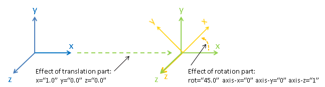
Location-element-transformation.png
Any rotation of a coordinate system can be performed by a rotation about some axis, however, sometime it may be advantageous to think of such a rotation as a composite of two or more rotations. For this reason a <location> element is allowed to have sub-rotation-elements, and an example of a composite rotation is
<location r="4.8" t="5.3" p="102.8" rot="-20.6" axis-x="0" axis-y="1" axis-z="0">
  <rot val="102.8">
    <rot val="50" axis-x="0" axis-y="1" axis-z="0" />
  </rot>
</location>
The outermost is applied first followed by the 2nd outermost operation and so on. In the above example this results in a -20.6 degree rotation about the y-axis followed by a 102.8 degree rotation about the z-axis (of the frame which has just be rotated by -20.6 degrees) and finally followed by another rotation about the y-axis, this time by 50 degrees. Note that the z-axis for the second rotation is implicit since no other axis information provided for the second rotation. This is hard-coded. The ISIS NIMROD instrument (NIM_Definition.xml) uses this feature.
The translation part of a <location> element can like the rotation part also be split up into a nested set of translations. This is demonstrated below
<location  r="10" t="90" >
  <trans r="8" t="-90" />
</location>
This combination of two translations: one moving 10 along the x-axis in the positive direction and the other in the opposite direction by 8 adds up to a total translation of 2 in the positive x-direction. This feature, for example, is useful when the positions of detectors are best described in spherical coordinates with respect to an origin different from the origin of the parent component. For example, say you have defined a <type name=”bank”> with contains 3 pixels. The centre of the bank is at the location r=”1” with respect to the sample and the positions of the 3 pixels are known with respect to the sample to be at r=”1” and with t=”-1”, t=”0” and t=”1”. One option is to describe this bank/pixels structure as
<component type="bank">
  <location />
</component>

<type name="bank">
  <component type="pixel">
    <location r="1" t="-1" />
    <location r="1" t="0" />
    <location r="1" t="1" />
  </component>
</type>
However a better option for this case is to use nested translations as demonstrated below
<component type="bank">
  <location r="1"/>
</component>

<type name="bank">
  <component type="pixel">
    <location r="1" t="180"> <trans r="1" t="-1" /> </location>
    <location r="1" t="180"> <trans r="1" t="0" /> </location>
    <location r="1" t="180"> <trans r="1" t="1" /> </location>
  </component>
</type>
since this means the bank is actually specified at the right location, and not artificially at the sample position.
Finally a combination of <trans> and <rot> sub-elements of a <location> element can be used as demonstrated below
<location x="10" >
  <rot val="90" >
    <trans x="-8" />
  </rot>
</location>
which put something at the location (x,y,z)=(10,-8,0) relative to the parent component and with a 90 rotation around the z-axis, which causes the x-axis to be rotated onto the y-axis.
Most of the attributes of have default values. These are: x=”0” y=”0” z=”0” rot=”0” axis-x=”0” axis-y=”0” axis-z=”1”
The <facing> element is an element you can use together with a <location>. Its purpose is to be able, with one line of IDF code, to make a given component face a point in space. For example many detectors on ISIS instruments are setup to face the sample. A <facing>element must be specified as a sub-element of a <location> element, and the facing operation is applied after the translation and/or rotation operation as specified by the location element. An example of a <facing> element is
<facing x="0.0" y="0.0" z="0.0"/>
or
<facing r="0.0" t="0.0" p="0.0"/>
In addition if the <components-are-facing> is set under <defaults>, i.e. by default any component in the IDF will be rotated to face a default position then
<facing val="none"/>
can be used to overwrite this default to say you don’t want to apply ‘facing’ to given component.
The process of facing is to make the xy-plane of the geometric shape of the component face the position specified in the <facing> element. The z-axis is normal to the xy-plan, and the operation of facing is to change the direction of the z-axis so that it points in the direction from the position specified in the facing <facing> towards the position of the component.
<facing> supports a rot attribute, which allow rotation of the z-axis around it own axis before changing its direction. The effect of rot here is identical to the effect of using rot in a <location> where axis-x=”0.0” axis-y=”0.0” axis-z=”1.0”. Allowing rot here perhaps make it slightly clearly that such a rot is as part of facing a component towards another component.
which rotate the is a convenient element for adjusting the orientation of the z-axis. The base rotation is to take the direction the z-axis points and change it to point from the position specified by the <facing> element to the position of the component.
A <location> specifies the location of a <type>. If this type consists of a number of sub-parts <exclude> can be used to exclude certain parts of a type. For example say the type below is defined in an IDF
<type name="door">
  <component type="standard-tube">
    <location r="2.5" t="19.163020" name="tube1"/>
    <location r="2.5" t="19.793250" name="tube2"/>
    <location r="2.5" t="20.423470" name="tube3"/>
    <location r="2.5" t="21.053700" name="tube4"/>
    <location r="2.5" t="21.683930" name="tube5"/>
  </component>
</type>
and the instrument consists of a number of these doors but where some of the doors are different in the sense that for example the 1st and/or the 2nd tube is missing from some of these. Using <exclude> this can be succinctly described as follows:
<component type="door">
  <location x="0">
    <exclude sub-part="tube1"/>
    <exclude sub-part="tube3"/>
  </location>
  <location x="1" />
  <location x="2" />
  <location x="3">
    <exclude sub-part="tube3"/>
  </location>
</component>
where the sub-part of refers to the ‘name’ of a part of the type ‘door’.
Most instruments have detectors which are ordered in some way. For a rectangular array of detectors we have a shorthand notation. The <locations> tag is a shorthand notation to use for a linear/spherical sequence of detectors, as any of the position coordinates or the coordinate rotation angles of a <location> tag are changing.
For example a <locations> element may be used to describe the position of equally distanced pixels along a tube, in the example below along the y variable
<locations y="1.0" y-end="10.0" n-elements="10" name="det"/>
The above one line of XML is shorthand notation for
<location y="1.0" name="det0"/>
<location y="2.0" name="det1" />
<location y="3.0" name="det2" />
<location y="4.0" name="det3" />
<location y="5.0" name="det4" />
<location y="6.0" name="det5" />
<location y="7.0" name="det6" />
<location y="8.0" name="det7" />
<location y="9.0" name="det8" />
<location y="10.0" name="det9" />
As is seen n-elements is the number of <location> elements this <locations> element is shorthand for. y-end specifies the y end position, and the equal distance in y between the pixels is calculated in the code as (‘y’-‘y-end’)/(‘n-elements’-1). Multiple ‘variable’-end attributes can be specified for the <locations> tag, where ‘variable’ here is any of the <location> attributes: x, y, z, r, t, p and rot. The example below describes a list of detectors aligned in a semi-circle:
<locations n-elements="7" r="0.5" t="0.0" t-end="180.0" rot="0.0" rot-end="180.0" axis-x="0.0" axis-y="1.0" axis-z="0.0"/>
The above one line of XML is shorthand notation for
<location r="0.5" t="0"   rot="0"   axis-x="0.0" axis-y="1.0" axis-z="0.0"/>
<location r="0.5" t="30"  rot="30"  axis-x="0.0" axis-y="1.0" axis-z="0.0"/>
<location r="0.5" t="60"  rot="60"  axis-x="0.0" axis-y="1.0" axis-z="0.0"/>
<location r="0.5" t="90"  rot="90"  axis-x="0.0" axis-y="1.0" axis-z="0.0"/>
<location r="0.5" t="120" rot="120" axis-x="0.0" axis-y="1.0" axis-z="0.0"/>
<location r="0.5" t="150" rot="150" axis-x="0.0" axis-y="1.0" axis-z="0.0"/>
<location r="0.5" t="180" rot="180" axis-x="0.0" axis-y="1.0" axis-z="0.0"/>
If name is specified, e.g. as name=”det” in the first example, then as seen the <location> elements are given the ‘name’ plus a counter, where by default this counter starts from zero. This counter can optionally be changed by using attribute name-count-start, e.g. setting name-count-start=”1” in the above example would have named the 10 <location> elements det1, det2, …, det10. Additionally, using the name-count-increment attribute, e.g setting name-count-increment=”2” would have named the 10 <location> elements dat1, det3, …, det21. By default, this increment is one.
When one <locations> tag was used in ISIS LET_Definition.xml the number of lines of this file reduced from 1590 to 567.
Parameters which do not change or are changed via <logfile> should be stored using this element inside the IDF, however parameters which may need to be accessed and changed manually on a regular basis should be stored in a separate parameter file.
<parameter> is used to specify a value to a parameter which can then be extracted from Mantid. One usage of <parameter> is to link values stored in log-files to parameter names. For example
<parameter name="x">
  <logfile id="trolley2_x_displacement" extract-single-value-as="position 1" />
</parameter>
reads: “take the first value in the “trolley2_x_displacement” log-file and use this value to set the parameter named ‘x’.
The name of the <parameter> is specified using the ‘name’ tag. You may specify any name for a parameter except for name=”pos” and name=”rot”. These are reserved keywords. Further a few names have a special effect when processed by Mantid
The value of the parameter is in the above example specified using a log-file as specified with the element <logfile>. The required attribute of <logfile> is
Optional attributes of <logfile> are:
Another option for specifying a value for a parameter is to use the notation:
<parameter name="x">
  <value val="7.2"/>
</parameter>
Here a value for the parameter with name “x” is set directly to 7.2. The only and required attribute of the <value> element is ‘val’.
For a given <parameter> you should specify its value only once. If by mistake you specify a value twice as demonstrated in the example below then the first encountered <value> element is used, and if no <value> element is present then the first encountered <logfile> element is used.
<parameter name="x">
  <value val="7.2"/>
  <logfile id="trolley2_x_displacement" extract-single-value-as="position 1" />
</parameter>
In the above example <value val=”7.2”/> is used.
Parameters are by default accessed recursively. Demonstrated with an example:
<component type="dummy">
  <location/>
  <parameter name="something"> <value val="35.0"/> </parameter>
</component>

<type name="dummy">
  <component type="pixel" name="pixel1">
    <location y="0.0" x="0.707" z="0.707"/>
    <parameter name="something1"> <value val="25.0"/> </parameter>
  </component>

  <component type="pixel" name="pixel2">
    <location y="0.0" x="1.0" z="0.0"/>
    <parameter name="something2"> <value val="15.0"/> </parameter>
  </component>
</type>
this implies that if you for instance ask the component with name=”pixel1” what parameters it has then the answer is two: something1=25.5 and something=35.0. If you ask the component name=”dummy” the same question the answer is one: something=35.0 and so on.
This is a special category of parameters where the value specified for the parameter is string rather than a double. The syntax is
<parameter name="instrument-status" type="string">
  <value val="closed"/>
</parameter>
This is a special category of parameters, which follows the same syntax as other but allows a few extra features. Fitting parameters are meant to be used when raw data are fitted against models that contain parameters, where some of these parameters are instrument specific. If such parameters are specified these will be pulled in before the fitting process starts, where optionally these may, for instance, be specified to be treated as fixed by default. To specify a fitting parameter use the additional tag type=”fitting” as shown in the example below
<parameter name="IkedaCarpenterPV:Alpha0" type="fitting">
  <value val="7.2"/>
</parameter>
It is required that the parameter name uses the syntax NameOfFunction:Parameter, where NameOfFunction is the name of the fitting function the parameter is associated with. In the example above the fitting function name is IkedaCarpenterPV and the parameter name is Alpha0.
To specify that a parameter should be treated as fixed in the fitting process use the element as demonstrated in the example below
<parameter name="IkedaCarpenterPV:Alpha0" type="fitting">
  <value val="7.2"/>
  <fixed />
</parameter>
A parameter can be specified to have a min/max value, which results in a constraint being applied to this parameter. An example of this is shown below
<parameter name="IkedaCarpenterPV:Alpha0" type="fitting">
  <value val="7.2"/>
  <min val="4"/> <max val="12"/>
</parameter>
The min/max values may also be specified as percentage values. For example:
<parameter name="IkedaCarpenterPV:Alpha0" type="fitting">
  <value val="250"/>
  <min val="80%"/> <max val="120%"/>
  <penalty-factor val="2000"/>
</parameter>
results in Alpha0 being constrained to sit between 250*0.8=200 and 250*1.20=300. Further this example also demonstrates how a can be specified to tell how strongly the min/max constraints should be enforced. The default value for the penalty-factor is 1000. For more information about this factor see FitConstraint.
A value for a parameter may alternatively be set using a look-up-table or a formula. An example demonstrating a formula is
<parameter name="IkedaCarpenterPV:Alpha0" type="fitting">
  <formula eq="100.0+10*centre+centre^2" unit="TOF" result-unit="1/dSpacing^2"/>
</parameter>
‘centre’ in the formula is substituted with the centre-value of the peak shape function as known prior to the start of the fitting process. The attributes ‘unit’ is optional. If it is not set then the peak centre-value is directly substituted for the centre variable in the formula. If it is set then it must be set to no one of the units defined in Unit Factory, and what happens is that the peak centre-value is converted to this unit before assigned to the centre variable in the formula.
The optional ‘result-unit’ attribute tells what the unit is of the output of the formula. In the example above this unit is “1/dSpacing^2” (for the ‘result-unit’ this attribute can be set to an algebraic expression of the units defined in Unit Factory). If the x-axis unit of the data you are trying to fit is dSpacing then the output of the formula is left as it is. But for example if the x-axis unit of the data is TOF then the formula output is converted into, it in this case, the unit “1/TOF^2”. Examples where ‘unit’ and ‘result-unit’ are used include: CreateBackToBackParameters and CreateIkedaCarpenterParameters.
An example which demonstrate using a look-up-table is
<parameter name="IkedaCarpenterPV:Alpha0" type="fitting">
  <lookuptable interpolation="linear" x-unit="TOF" y-unit="dSpacing">
    <point x="1" y="1" />
    <point x="3" y="100" />
    <point x="5" y="1120" />
    <point x="10" y="1140" />
  </lookuptable>
</parameter>
As with a formula the look-up is done for the ‘x’-value that corresponds to the centre of the peak as known prior to the start of the fitting process. The only interpolation option currently supported is ‘linear’. The optional ‘x-unit’ and ‘y-unit’ attributes must be set to one of the units defined in Unit Factory. The ‘x-unit’ and ‘y-unit’ have very similar effect to the ‘unit’ and ‘result-unit’ attributes for described above. ‘x-unit’ converts the unit of the centre before lookup against the x-values. ‘y-axis’ is the unit of the y values listed, which for the example above correspond to Alpha0.
Allow <parameter>s to be linked to components without needing <parameter>s to be defined inside, as sub-elements, of the components they belong to. The standard approach for defining a parameter is
<component type="bank" name="bank_90degnew">
  <location />
  <parameter name="test"> <value val="50.0" /> </parameter>
</component>
where a parameter ‘test’ is defined to belong to the component with the name ‘bank_90degnew’. However, alternatively the parameter can be defined using the notation in the an example below. Note that if more than one component e.g. have the name ‘bank_90degnew’ then the specified parameters are applied to all such components.
<component type="bank" name="bank_90degnew">
  <location />
</component>

<component-link name="bank_90degnew" >
  <parameter name="test"> <value val="50.0" /> </parameter>
</component-link>
<component-link> is the only way parameters can be defined in a parameter file used by the LoadParameterFile algorithm.
If there are several components with name ‘bank_90degnew’ but you want specified paramentes to apply to only one of them, then you can specify the name by a path name.
<component-link name="HRPD/leftside/bank_90degnew" >
  <parameter name="test"> <value val="50.0" /> </parameter>
</component-link>
The path name need not be complete provided it specifies a unique component. Here we drop the instrument name HRPD.
<component-link name="leftside/bank_90degnew" >
  <parameter name="test"> <value val="50.0" /> </parameter>
</component-link>
The standard way of making up geometric shapes as a collection of parts is described here: HowToDefineGeometricShape. However, <combine-components-into-one-shape> offers in some circumstances a more convenient way of defining more complicated shapes, as for example is the case for the ISIS POLARIS instrument. This tag combining components into one shape as demonstrated below:
<component type="adjusted cuboid">
  <location />
</component>

<type name="adjusted cuboid" is="detector">
  <combine-components-into-one-shape />
  <component type="cuboid1">
    <location name="A"/>
    <!-- "A" translated by y=10 and rotated around x-axis by 90 degrees -->
    <location name="B" y="10" rot="90" axis-x="1" axis-y="0" axis-z="0" />
  </component>
  <algebra val="A : B" />

  <!-- this bounding box is used for this combined into one shape-->
  <bounding-box>
    <x-min val="-0.5"/>
    <x-max val="0.5"/>
    <y-min val="-5.0"/>
    <y-max val="10.5"/>
    <z-min val="-5.0"/>
    <z-max val="5.0"/>
  </bounding-box>

</type>

<type name="cuboid1" is="detector">
  <cuboid id="bob">
    <left-front-bottom-point x="0.5" y="-5.0" z="-0.5"  />
    <left-front-top-point  x="0.5" y="-5.0" z="0.5"  />
    <left-back-bottom-point  x="-0.5" y="-5.0" z="-0.5"  />
    <right-front-bottom-point  x="0.5" y="5.0" z="-0.5"  />
  </cuboid>

  <!-- this bounding box is not used in the combined shape -->
  <!-- Note you would not normally need to add a bounding box
       for a single cuboid shape. The reason for adding one
       here is just to illustrate that a bounding added here
       will not be used in created a combined shape as in
       "adjusted cuboid" above -->
  <bounding-box>
    <x-min val="-0.5"/>
    <x-max val="0.5"/>
    <y-min val="-5.0"/>
    <y-max val="5.0"/>
    <z-min val="-0.5"/>
    <z-max val="0.5"/>
  </bounding-box>
</type>
which combines two components “A” and “B” into one shape. The resulting shape is shape is shown here:
CombineIntoOneShapeExample.png
Note for this to work, a unique name for each component must be provided and these names must be used in the algebra string (here “A : B”, see HowToDefineGeometricShape). Further a bounding-box may optionally be added to the to the type. Note the above geometric shape can alternatively be defined with the XML (Mantid behind the scene translates the above XML to the XML below before proceeding):
<component type="adjusted cuboid">
  <location />
</component>

<type name="adjusted cuboid" is="detector">
  <cuboid id="A">
    <left-front-bottom-point x="0.5" y="-5.0" z="-0.5"  />
    <left-front-top-point  x="0.5" y="-5.0" z="0.5"  />
    <left-back-bottom-point  x="-0.5" y="-5.0" z="-0.5"  />
    <right-front-bottom-point  x="0.5" y="5.0" z="-0.5"  />
  </cuboid>
  <!-- cuboid "A" translated along y by 10 and rotated around x by 90 degrees -->
  <cuboid id="B">
    <left-front-bottom-point x="0.5" y="10.5" z="-5.0"  />
    <left-front-top-point  x="0.5" y="9.5" z="-5.0"  />
    <left-back-bottom-point  x="-0.5" y="9.5" z="-5.0"  />
    <right-front-bottom-point  x="0.5" y="10.5" z="5.0"  />
  </cuboid>
  <algebra val="A : B" />
</type>
<combine-components-into-one-shape> for now works only for combining cuboids. Please do not hesitate to contact the Mantid team if you would like to extend this.
This applies when defining any geometric shape, but perhaps something which a user has to be in particular aware of when defining more complicated geometry shapes, for example, using the <combine-components-into-one-shape> tag: the coordinate system in which a shape is defined can be chosen arbitrary, and the origin of this coordinate system is the position returned when a user asked for its position. It is therefore highly recommended that when a user define a detector geometric shape, this could be simple cuboid, that it is defined with the origin at the centre of the front of the detector. For detector shapes build up of for example multiple cuboids the origin should be chosen perhaps for the center of the front face of the ‘middle’ cuboid. When Mantid as for the position of such a shape it will be with reference to coordinate system origin of the shape. However, sometimes it may simply be inconvenient to build up a geometry shape with an coordinate system as explained above. For this case, and for now only when using <combine-components-into-one-shape> it possible to get around this by using the element <translate-rotate-combined-shape-to>, which takes the same attributes as a <location> element. The effect of this element is basically to redefine the shape coordinate system origin (in fact also rotate it if requested).
Used for setting various defaults.
Used to make the xy-plane of the geometric shape of any component by default face a given location. For example
<components-are-facing x="0.0" y="0.0" z="0.0" />
If this element is not specified the default is to not attempt to apply facing.
Originally introduced to handle detector position coordinates as defined by the Ariel software.
<offsets spherical="delta" />
When this is set all components which have coordinates specified using spherical coordinates (i.e. using the r, t, p attributes, see description of <location>) are then treated as offsets to the spherical position of the parent, i.e. the value given for \(r\) are added to the parent’s \(r\) to give the total radial coordinate, and the same for \(\theta\) and \(\phi\). Note using this option breaks the symmetry that the <location> element of a child component equals the position of this component relative to its parent component.
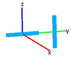
Reference frame in which instrument is described. The author/reader of an IDF can chose the reference coordinate system in which the instrument is described. The default reference system is the one shown below. The direction here means the direction of the beam if it was not modified by any mirrors etc.
<reference-frame>
  <!-- The z-axis is set parallel to and in the direction of the beam. the
       y-axis points up and the coordinate system is right handed. -->
  <along-beam axis="z"/>
  <pointing-up axis="y"/>
  <handedness val="right"/>
</reference-frame>
This reference frame is e.g. used when a signed theta detector values are calculated where it is needed to know which direction is defined as up. By default, the axis defining the sign of the scattering angle is the one pointing up. Optionally this can be customized by inserting the following line into the reference-frame node:
<theta-sign axis="x"/>
In this case, negative x will correspond to negative theta. Note that both the pointing-up and theta-sign axes cannot be the same as the along-beam axis.
This tag is used to control how the instrument first appears in the
Instrument View. Attribute view
defines the type of the view that opens by default. It can have the
following values: “3D”, “cylindrical_x”, “cylindrical_y”,
“cylindrical_z”, “spherical_x”, “spherical_y”, “spherical_z”. If the
attribute is omitted value “3D” is assumed. Opening the 3D view on
start-up is also conditioned on the value of the
MantidOptions.InstrumentView.UseOpenGL property in the Properties
File. If set to “Off” this property prevents the
Instrument View to start in 3D mode and “cylindrical_y” is used
instead. The user can change to 3D later.
Another attribute, axis-view governs on which axis the instrument is
initially viewed from in 3D and can be set equal to one of “Z-“, “Z+”,
“X-“, etc. If “Z-” were selected then the view point would be on the
z-axis on the negative of the origin looking in the +z direction.
If
<angle unit="radian"/>
is set then all angles specified in <location> elements and <parameter>’s with names “rotx”, “roty”, “rotz”, “t-position” and “p-position” are assumed to in radians. The default is to assume all angles are specified in degrees.
<length unit="meter"/>
This default, for now, does not do anything, but is the default unit for length used by Mantid. If it would be useful for you to specify user defined units do not hesitate to request this.
To prevent an IDF file from getting too long and complicated, information not related to the geometry of the instrument may be put into a separate file, whose content is automatically included into the IDF file.
For more information see the parameter file page.
The following features are now deprecated and should no longer be used.
mark-as=”monitor”
The following notation to mark a detector as a monitor is now deprecated:
<component type="monitor" idlist="monitor">
    <location r="3.25800" t="180.0" p="0.0" mark-as="monitor"/>
</component>

<type name="monitor" is="detector"/>

<idlist idname="monitor">
  <id val="11" />
</idlist>
The above XML should be replaced with
<component type="monitor" idlist="monitor">
    <location r="3.25800" t="180.0" p="0.0"/>
</component>

<type name="monitor" is="monitor"/>

<idlist idname="monitor">
  <id val="11" />
</idlist>
Category: Concepts