The Tabs - Results#
Results#
The Results tab allows the user to:
Create a result(s) table.
Select which instrument log values (temp, field etc) to write out alongside the fit parameters.
Choose to write out fit information from one or several data files.
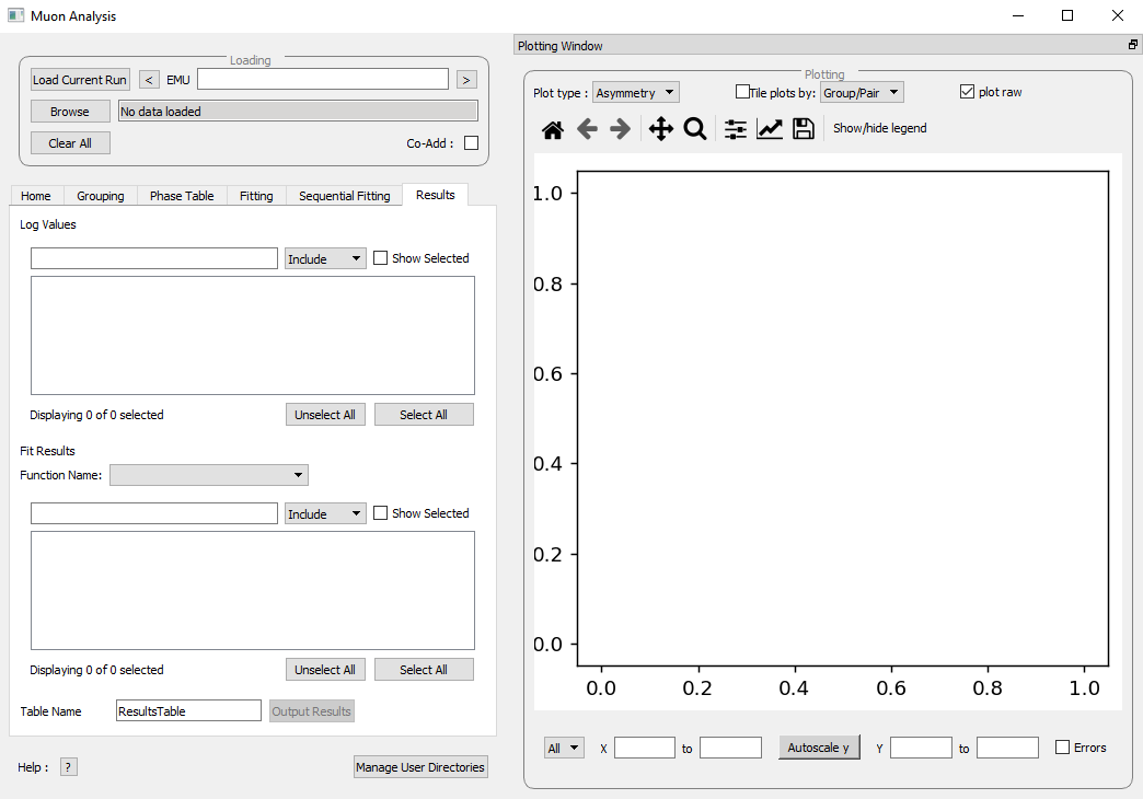
Figure 32: The Results tab options.#
The user has chosen to create a results table. When the ‘Output Results’ button is clicked, the resulting table will appear in the ADS. From here the data can be explored and plotted as one would with any data in a Mantid workspace. The data contained in a results table is determined by the contents of the Values and Fitting Results sections (in the example above these are empty; no data has been fitted, so there are no workspaces available for the Fitting Results section).
In the Values sections, the user can choose which Log Values to include in the results table, these values are data from the instrument such as run number, sample temperature etc. and are taken from the workspaces in the Fitting Results section.
NB even if a workspace from the Fit Result table has not been selected (via the checkbox), the types of Log Value it contains will still be present in the Values table. This does not mean they will be included in a produced results table.
The Fit Results section allows the user to choose which workspaces to use Log Values from - these can be either individual fits, or a sequential/simultaneous fits. The first option in this section is the Function Name drop-down menu, selecting a certain function in this menu will show all the workspaces that have had this function fitted to them in the table below. By default, checking the box next to a workspace in this table means its Log Values will be present in the results table. This can be changed with the Include/Exclude option (if Exclude is selected from the drop-down menu, checked workspaces will be the only ones not included in the table). The view can also be customised to only show selected workspaces.
As an exercise, follow the instructions below in order to produce a results table for a single individual or sequential fit.
Load the HIFI00062798 file from the reference folder, guess \(\alpha\) as described in grouping then fit the ExpDecayOsc function to it. To demonstrate a sequential fit table, load the EMU00019631-4 files, don’t guess \({\alpha}\), and then perform a sequential fit of ExpDecayOsc on those files. (See using fit functions for instructions on single and sequential fits.)
In the Results tab, the default individual fit table should already be set up. Check that the Function Name and workspace(s) selected in the lower part of the tab show the fit function and data used so far, respectively.
Use the table in the Log Values section to select parameters to include in the results table. This is done by checking the box next to them - try this now for run number and Temp_Sample.
Pick a name for the table, then click Output Results. See figure 33 for the process for an individual fit, and 34 for sequential.
To view a table, right click it in the ADS and then select Show Data.
Figure 33: How to create a results table from a single individual fit.#
Figure 34: How to create a results table from a sequential fit.#
Plotting from a Results Table#
Once a results table has been created, there are now different sets of parameters available for individual analysis. In Mantid, it is possible to plot different parameters against each other, to see the relationship between the two.
Follow the instructions below in order to plot a graph from parameters in a Results Table.
Files EMU00019631.nxs to EMU00019634.nxs should already have been loaded, sequentially fitted and a Results Table produced from them during the last section. If not then load the files, fit and produce a table.
This example plots Temp_Sample against Lambda, which should automatically be assigned to the X and Y axes by Mantid (labelled X1 and Y1 respectively) click on Temp_Sample to select it.
NB If data is not automatically assigned to the desired axes this can be changed manually. As an example, if in step 2. `Temp_Sample` was not already assigned to X, it could be right clicked after selection and then `Set as X`. This process is shown in 35. There are also other options such as to assign data to the `Y` axis, or `Y error`.
Next, hold down the Ctrl key and click on the Lambda column to select this column as well as Temp_Sample.
Right click one of the columns and follow Plot > Line and Symbol. This will bring up a plot of Temp_Sample on the X axis and Lambda on the Y axis. See Figure 35 for the process.
The axis titles may not be entirely correct, so it may be best to change them. To do this, just double click the title and re-write it.
Figure 35: How to plot a graph from two parameters of a results table.#
For more details on the Results tab, see the corresponding section of Muon Analysis